travel method is

• View source
• View history
• Community portal
• Recent changes
• Random page
• Featured content
• What links here
• Related changes
• Special pages
• Printable version
• Permanent link
• Page information
• Browse properties

Travel cost method

This article deals with the Travel Cost Method, which is often used in evaluating the economic value of recreational sites. This is particularly important in the coastal zone because of the level of use and the potential values that can be attached to the natural coastal and marine environment.

The Travel Cost Method (TCM) is one of the most frequently used approaches to estimating the use values of recreational sites. The TCM was initially suggested by Hotelling [1] and subsequently developed by Clawson [2] in order to estimate the benefits from recreation at natural sites. The method is based on the premise that the recreational benefits at a specific site can be derived from the demand function that relates observed users’ behaviour (i.e., the number of trips to the site) to the cost of a visit. One of the most important issues in the TCM is the choice of the costs to be taken into account. The literature usually suggests considering direct variable costs and the opportunity cost of time spent travelling to and at the site. The classical model derived from the economic theory of consumer behaviour postulates that a consumer’s choice is based on all the sacrifices made to obtain the benefits generated by a good or service. If the price ( [math]p[/math] ) is the only sacrifice made by a consumer, the demand function for a good with no substitutes is [math]x=f(p)[/math] , given income and preferences. However, the consumer often incurs other costs ( [math]c[/math] ) in addition to the out-of-pocket price, such as travel expenses, and loss of time and stress from congestion. In this case, the demand function is expressed as [math]x = f(p, c)[/math] . In other words, the price is an imperfect measure of the full cost incurred by the purchaser. Under these conditions, the utility maximising consumer’s behaviour should be reformulated in order to take such costs into account. Given two goods or services [math]x_1, x_2[/math] , their prices [math]p_1, p_2[/math] , the access costs [math]c_1, c_2[/math] and income [math]R[/math] , the utility maximising choice of the consumer is:

[math]max \, U = u(x_1,x_2) \quad subject \, to \quad (p_1+c_1)x_1+(p_2+c_2)x_2=R . \qquad (1)[/math]

Now, let [math]x_1[/math] denote the aggregate of priced goods and services, [math]x_2[/math] the number of annual visits to a recreational site, and assume for the sake of simplicity that the cost of access to the market goods is negligible ( [math]c_1 \approx 0[/math] ) and that the recreational site is free ( [math]p_2=0[/math] ). Under these assumptions, equation (1) can be written as:

[math]max \, U = u(x_1,x_2) \quad subject \, to \quad p_1x_1+c_2x_2=R . \qquad (2)[/math]

Under these conditions, the utility maximising behaviour of the consumer depends on:

The TCM is based on the assumption that changes in the costs of access to the recreational site [math]c_2[/math] have the same effect as a change in price: the number of visits to a site decreases as the cost per visit increases. Under this assumption, the demand function for visits to the recreational site is [math]x_2=f(c_2)[/math] and can be estimated using the number of annual visits as long as it is possible to observe different costs per visit. The basic TCM model is completed by the weak complementarity assumption, which states that trips are a non-decreasing function of the quality of the site, and that the individual forgoes trips to the recreational site when the quality is the lowest possible [3] , [4] . There are two basic approaches to the TCM: the Zonal approach (ZTCM) and the Individual approach (ITCM). The two approaches share the same theoretical premises, but differ from the operational point of view. The original ZTCM takes into account the visitation rate of users coming from different zones with increasing travel costs. By contrast, ITCM, developed by Brown and Nawas [5] and Gum and Martin [6] , estimates the consumer surplus by analysing the individual visitors’ behaviour and the cost sustained for the recreational activity. These are used to estimate the relationship between the number of individual visits in a given time period, usually a year, the cost per visit and other relevant socio-economic variables. The ITCM approach can be considered a refinement or a generalisation of ZTCM [7] .

[math]x_2 = g(c_2) . \qquad (3)[/math]

The demand function can also be estimated for non-homogeneous sub-samples introducing among the independent variables income and socio-economic variables representing individual characteristics [8] . Therefore, if an individual incurs [math]c_2^e[/math] per visit, he chooses to do [math]x_2^e[/math] visits a year, while if the cost per visit increases to [math]c_2^p[/math] the number of visits will decrease to [math]x_2^p[/math] . The cost [math]cp[/math] is the choke price, that is the cost per visit that results in zero visits. The annual user surplus (the use value of the recreational site) is easily obtained by integrating the demand function from zero to the current number of annual visits, and subtracting the total expenditures on visits.

Related articles

• ↑ Hotelling, H. (1949), Letter, In: An Economic Study of the Monetary Evaluation of Recreation in the National Parks , Washington, DC: National Park Service.
• ↑ Clawson, M. (1959), Method for Measuring the Demand for, and Value of, Outdoor Recreation . Resources for the Future, 10, Washington, DC.
• ↑ Freeman, A.M. III. (1993). The Measurement of Environmental and Resource Values: Theory and Method , Washington, DC: Resources for the Future.
• ↑ Herriges, J.A., C. Kling and D.J. Phaneuf (2004), 'What’s the Use? Welfare Estimates from Revealed Preference Models when Weak Complementarity Does Not Hold', Journal of Environmental Economics and Management , 47 (1), pp. 53-68.
• ↑ Brown, W.G. and F. Nawas (1973), 'Impact of Aggregation on the Estimation of Outdoor Recreation Demand Functions', American Journal of Agricultural Economics , 55, 246-249.
• ↑ Gum, R.L. and W.E.Martin (1974), 'Problems and Solutions in Estimating the Demand for and Value of Rural Outdoor Recreation', American Journal of Agricultural Economics , 56, 558-566.
• ↑ Ward, F.A. and D. Beal (2000), Valuing Nature with Travel Cost Method: A Manual , Northampton: Edward Elgar.
• ↑ Hanley, N. and C.L. Spash (1993), Cost Benefit Analysis and the Environment , Aldershot, UK: Edward Elgar.
• Definitions
• Articles by Paolo Rosato
• Integrated coastal zone management
• Evaluation and assessment in coastal management
• This page was last edited on 3 March 2022, at 21:18.
• Privacy policy
• About Coastal Wiki
• Disclaimers

Environmental Justice Organisations, Liabilities and Trade

Mapping environmental justice.

• Nuclear Energy
• Oil and Gas and Climate Justice
• Biomass and Land Conflicts
• Mining and Ship Breaking
• Environmental Health and Risk Assessment
• Liabilities and Valuation
• Law and Institutions
• Consumption, Ecologically Unequal Exchange and Ecological Debt

Travel-cost method

The travel-cost method (TCM) is used for calculating economic values of environmental goods. Unlike the contingent valuation method, TCM can only estimate use value of an environmental good or service. It is mainly applied for determining economic values of sites that are used for recreation, such as national parks. For example, TCM can estimate part of economic benefits of coral reefs, beaches or wetlands stemming from their use for recreational activities (diving and snorkelling/swimming and sunbathing/bird watching). It can also serve for evaluating how an increased entrance fee a nature park would affect the number of visitors and total park revenues from the fee. However, it cannot estimate benefits of providing habitat for endemic species.

TCM is based on the assumption that travel costs represent the price of access to a recreational site. Peoples’ willingness to pay for visiting a site is thus estimated based on the number of trips that they make at different travel costs. This is called a revealed preference technique, because it ‘reveals’ willingness to pay based on consumption behaviour of visitors.

The information is collected by conducting a survey among the visitors of a site being valued. The survey should include questions on the number of visits made to the site over some period (usually during the last 12 months), distance travelled from visitor’s home to the site, mode of travel (car, plane, bus, train, etc.), time spent travelling to the site, respondents’ income, and other socio-economic characteristics (gender, age, degree of education, etc). The researcher uses the information on distance and mode of travel to calculate travel costs. Alternatively, visitors can be asked directly in a survey to state their travel costs, although this information tends to be somewhat less reliable. Time spent travelling is considered as part of the travel costs, because this time has an opportunity cost. It could have been used for doing other activities (e.g. working, spending time with friends or enjoying a hobby). The value of time is determined based on the income of each respondent. Time spent at the site is for the same reason also considered as part of travel costs. For example, if respondents visit three different sites in 10 days and spend only 1 day at the site being valued, then only fraction of their travel costs should be assigned to this site (e.g. 1/10). Depending on the fraction used, the final benefit estimates can differ considerably.

Two approaches of TCM are distinguished – individual and zonal. Individual TCM calculates travel costs separately for each individual and requires a more detailed survey of visitors. In zonal TCM, the area surrounding the site is divided into zones, which can be either concentric circles or administrative districts. In this case, the number of visits from each zone is counted. This information is sometimes available (e.g. from the site management), which makes data collection from the visitors simpler and less expensive.

The relationship between travel costs and number of trips (the higher the travel costs, the fewer trips visitors will take) shows us the demand function for the average visitor to the site, from which one can derive the average visitor’s willingness to pay. This average value is then multiplied by the total relevant population in order to estimate the total economic value of a recreational resource.

TCM is based on the behaviour of people who actually use an environmental good and therefore cannot measure non-use values. This method is thus inappropriate for sites with unique characteristics which have a large non-use economic value component (because many people would be willing to pay for its preservation just to know that it exists, although they do not plan to visit the site in the future).

The travel-cost method might also be combined with contingent valuation to estimate an economic value of a change (either enhancement or deterioration) in environmental quality of the NP by asking the same tourists how many trips they would make in the case of a certain quality change. This information could help in estimating the effects that a particular policy causing an environmental quality change would have on the number of visitors and on the economic use value of the NP.

For further reading:

Ward, F.A., Beal, D. (2000) Valuing nature with travel cost models. A manual. Edward Elgar, Cheltenham.

Ecosystem valuation [ www.ecosystemvaluation.org/travel_costs.htm ]

This glossary entry is based on a contribution by Ivana Logar 

EJOLT glossary editors:   Hali Healy, Sylvia Lorek and Beatriz Rodríguez-Labajos

One comment

I quite like reading a post that will make people think. Also, thanks for allowing me to comment!

Browse by Theme

Browse by type.

• Presentations
• Press Releases
• Scientific Papers

Online course

Online course on ecological economics: http://www.ejolt.org/2013/10/online-course-ecological-economics-and-activism/

Privacy Policy | Credits

What is The Travel Method?

Travel and Packing Guides for the Modern Traveler

The Travel Method is a collection of travel and packing guides for the modern traveler from first-hand experience.

We are a husband and wife team that collectively have visited over forty countries and traveled full-time together for over three years.

Experiencing new places and making memories is why so many of us travel. However, travel itself, when you factor in all the planning, logistics, and unforeseen circumstances, can be super stressful.

Our tips and guides, drawing on years of experience traveling all over the world, can help you plan better and travel smarter. If you have the right equipment, plan well, and proactively try to prepare for potential challenges, your trip should run much smoother. That frees you up to actually have a good time!

In addition, we also work closely with local writers and travel enthusiasts from particular countries. As locals, they can offer far more valuable insight into traveling to their home country than someone who, for example, only spent a couple of weeks there.

Dale Johnson

Dale is a writer and graphic designer who has traveled to and lived in over thirty countries to date, and traveled full-time for over three years. During that time, he also co-ran and organized retreats for digital nomads in several different countries.

This firsthand experience of not only traveling himself, but organizing travel experiences for others, opened his eyes to many of the challenges that come with travel.

Doina Johnson

Doina Johnson has traveled full-time for over three years and to over thirty countries. She writes on a number of travel-themed topics for the Travel Method and travel and food-themed topics for a number of other publications.

Contributors

Roxana Fanaru

Roxana is a journalist who has lived in Italy for over two decades and travels frequently around Europe. She has written for various publications in the lifestyle and travel niche and is a seasoned solo traveler.

Ana Perusquia

Ana Perusquia is a content writer from Mexico City. She has worked extensively on our Mexico-specific content, including our packing list and tips for traveling to Mexico.

Nandhini Parthib

Nandhini Parthib is an Indian content writer who is deeply passionate about Indian culture, travel, and cuisine. Her expert insight can be found in our India-specific content, including our packing list and tips for traveling to India.

Want to create or adapt books like this? Learn more about how Pressbooks supports open publishing practices.

Part III: Travel Demand Modeling

9 Introduction to Transportation Modeling: Travel Demand Modeling and Data Collection

Chapter overview.

Chapter 9 serves as an introduction to travel demand modeling, a crucial aspect of transportation planning and policy analysis. As explained in previous chapters, the spatial distribution of activities such as employment centers, residential areas, and transportation systems mutually influence each other. The utilization of travel demand forecasting techniques leads to dynamic processes in urban areas. A comprehensive grasp of travel demand modeling is imperative for individuals involved in transportation planning and implementation.

This chapter covers the fundamentals of the traditional four-step travel demand modeling approach. It delves into the necessary procedures for applying the model, including establishing goals and criteria, defining scenarios, developing alternatives, collecting data, and conducting forecasting and evaluation.

Following this chapter, each of the four steps will be discussed in detail in Chapters 10 through 13.

Learning Objectives

• Describe the need for travel demand modeling in urban transportation and relate it to the structure of the four-step model (FSM).
• Summarize each step of FSM and the prerequisites for each in terms of data requirement and model calibration.
• Summarize the available methods for each of the first three steps of FSM and compare their reliability.
• Identify assumptions and limitations of each of the four steps and ways to improve the model.

Introduction

Transportation planning and policy analysis heavily rely on travel demand modeling to assess different policy scenarios and inform decision-making processes. Throughout our discussion, we have primarily explored the connection between urban activities, represented as land uses, and travel demands, represented by improvements and interventions in transportation infrastructure. Figure 9.1 provides a humorous yet insightful depiction of the transportation modeling process. In preceding chapters, we have delved into the relationship between land use and transportation systems, with the houses and factories in the figure symbolizing two crucial inputs into the transportation model: households and jobs. The output of this model comprises transportation plans, encompassing infrastructure enhancements and programs. Chapter 9 delves into a specific model—travel demand modeling. For further insights into transportation planning and programming, readers are encouraged to consult the UTA OERtransport book, “Transportation Planning, Policies, and History.”

Travel demand models forecast how people will travel by processing thousands of individual travel decisions. These decisions are influenced by various factors, including living arrangements, the characteristics of the individual making the trip, available destination options, and choices regarding route and mode of transportation. Mathematical relationships are used to represent human behavior in these decisions based on existing data.

Through a sequential process, transportation modeling provides forecasts to address questions such as:

• What will the future of the area look like?
• What is the estimated population for the forecasting year?
• How are job opportunities distributed by type and category?
• What are the anticipated travel patterns in the future?
• How many trips will people make? ( Trip Generation )
• Where will these trips end? ( Trip Distribution )
• Which transportation mode will be utilized? ( Mode Split )
• What will be the demand for different corridors, highways, and streets? ( Traffic Assignment )
• Lastly, what impact will this modeled travel demand have on our area? (Rahman, 2008).

9.2 Four-step Model

According to the questions above, Transportation modeling consists of two main stages, regarding the questions outlined above. Firstly, addressing the initial four questions involves demographic and land use analysis, which incorporates the community vision collected through citizen engagement and input. Secondly, the process moves on to the four-step travel demand modeling (FSM), which addresses questions 5 through 8. While FSM is generally accurate for aggregate calculations, it may occasionally falter in providing a reliable test for policy scenarios. The limitations of this model will be explored further in this chapter.

In the first stage, we develop an understanding of the study area from demographic information and urban form (land-use distribution pattern). These are important for all the reasons we discussed in this book. For instance, we must obtain the current age structure of the study area, based on which we can forecast future birth rates, death, and migrations  (Beimborn & Kennedy, 1996).

Regarding economic forecasts, we must identify existing and future employment centers since they are the basis of work travel, shopping travel, or other travel purposes. Empirically speaking, employment often grows as the population grows, and the migration rate also depends on a region’s economic growth. A region should be able to generate new employment while sustaining the existing ones based upon past trends and form the basis for judgment for future trends (Mladenovic & Trifunovic, 2014).

After forecasting future population and employment, we must predict where people go (work, shop, school, or other locations). Land-use maps and plans are used in this stage to identify the activity concentrations in the study area. Future urban growth and land use can follow the same trend or change due to several factors, such as the availability of open land for development and local plans and  zoning ordinances (Beimborn & Kennedy, 1996). Figure 9.3 shows different possible land-use patterns frequently seen in American cities.

Land-use pattern can also be forecasted through the integration of land use and transportation as we explored in previous chapters.

Figure 9.3 above shows a simple structure of the second stage of FSM.

Once the number and types of trips are predicted, they are assigned to various destinations and modes. In the final step, these trips are allocated to the transportation network to compute the total demand for each road segment. During this second stage, additional choices such as the time of travel and whether to travel at all can be modeled using choice models (McNally, 2007). Travel forecasting involves simulating human behavior through mathematical series and calculations, capturing the sequence of decisions individuals make within an urban environment.

The first attempt at this type of analysis in the U.S. occurred during the post-war development period, driven by rapid economic growth. The influential study by Mitchell and Rapkin (1954) emphasized the need to establish a connection between travel and activities, highlighting the necessity for a comprehensive framework. Initial development models for trip generation, distribution, and diversion emerged in the 1950s, leading to the application of the four-step travel demand modeling (FSM) approach in a transportation study in the Chicago area. This model was primarily highway-oriented, aiming to compare new facility development and improved traffic engineering. In the 1960s, federal legislation mandated comprehensive and continuous transportation planning, formalizing the use of FSM. During the 1970s, scholars recognized the need to revise the model to address emerging concerns such as environmental issues and the rise of multimodal transportation systems. Consequently, enhancements were made, leading to the development of disaggregate travel demand forecasting and equilibrium assignment methods that complemented FSM. Today, FSM has been instrumental in forecasting travel demand for over 50 years (McNally, 2007; Weiner, 1997).

Initially outlined by Mannheim (1979), the basic structure of FSM was later expanded by Florian, Gaudry, and Lardinois (1988). Figure 9.3 illustrates various influential components of travel demand modeling. In this representation, “T” represents transportation, encompassing all elements related to the transportation system and its services. “A” denotes the activity system, defined according to land-use patterns and socio-demographic conditions. “P” refers to transportation network performance. “D,” which stands for demand, is generated based on the land-use pattern. According to Florian, Gaudry, and Lardinois (1988), “L” and “S” (location and supply procedures) are optional parts of FSM and are rarely integrated into the model.

A crucial aspect of the process involves understanding the input units, which are defined both spatially and temporally. Demand generates person trips, which encompass both time and space (e.g., person trips per household or peak-hour person trips per zone). Performance typically yields a level of service, defined as a link volume capacity ratio (e.g., freeway vehicle trips per hour or boardings per hour for a specific transit route segment). Demand is primarily defined at the zonal level, whereas performance is evaluated at the link level.

It is essential to recognize that travel forecasting models like FSM are continuous processes. Model generation takes time, and changes may occur in the study area during the analysis period.

Before proceeding with the four steps of FSM, defining the study area is crucial. Like most models discussed, FSM uses traffic analysis zones (TAZs) as the geographic unit of analysis. However, a higher number of TAZs generally yield more accurate results. The number of TAZs in the model can vary based on its purpose, data availability, and vintage. These zones are characterized or categorized by factors such as population and employment. For modeling simplicity, FSM assumes that trip-making begins at the center of a zone (zone centroid) and excludes very short trips that start and end within a TAZ, such as those made by bike or on foot.

Furthermore, highway systems and transit systems are considered as networks in the model. Highway or transit line segments are coded as links, while intersections are represented as nodes. Data regarding network conditions, including travel times, speeds, capacity, and directions, are utilized in the travel simulation process. Trips originate from trip generation zones, traverse a network of links and nodes, and conclude at trip attraction zones.

Trip Generation

Trip generation is the first step in the FSM model. This step defines the magnitude of daily travel in the study area for different trip purposes. It will also provide us with an estimate of the total trips to and from each zone, creating a trip production and attraction matrix for each trip’s purpose. Trip purposes are typically categorized as follows:

• Home-based work trips (work trips that begin or end at home),
• Home-based shopping trips,
• Home-based other trips,
• School trips,
• Non-home-based trips (trips that neitherbeginnorendathome),
• Trucktrips,and
• Taxitrips(Ahmed,2012).

Trip attractions are based on the level of employment in a zone. In the trip generation step, the assumptions and limitations are listed below:

• Independent decisions: Travel behavior is affected by many factors generated within a household; the model ignores most of these factors. For example, childcare may force people to change their travel plans.
• Limited trip purposes: This model consists of a limited number of trip purposes for simplicity, giving rise to some model limitations. Take shopping trips, for example; they are all considered in the same weather conditions. Similarly, we generate home-based trips for various purposes (banking, visiting friends, medical reasons, or other purposes), all of which are affected by factors ignored by the model.
• Trip combinations: Travelers are often willing to combine various trips into a chain of short trips. While this behavior creates a complex process, the FSM model treats this complexity in a limited way.
• Feedback, cause, and effect problems: Trip generation often uses factors that are a function of the number of trips. For instance, for shopping trip attractions in the FSM model, we assume they are a retail employment function. However, it is logical to assume how many customers these retail centers attract. Alternatively, we can assume that the number of trips a household makes is affected by the number of private cars they own. Nevertheless, the activity levels of families determine the total number of cars.

As mentioned, trip generation process estimations are done separately for each trip purpose. Equations 1 and 2 show the function of trip generation and attraction:

where Oi and Dj trip are generated and attracted respectively, x refers to socio-economic characteristics, and y refers to land-use properties.

Generally, FSM aggregates different trip purposes previously listed into three categories: home-based work trips (HBW) , home-based other (or non-work) trips (HBO) , and non-home-based trips (NHB) . Trip ends are either the origin (generation) or destination (attraction), and home-end trips comprise most trips in a study area. We can also model trips at different levels, such as zones, households, or person levels (activity-based models). Household-level models are the most common scale for trip productions, and zonal-level models are appropriate for trip attractions (McNally, 2007).

There are three main methods for a trip generation or attraction.

• The first method is multiple regression based on population, jobs, and income variables.
• The second method in this step is experience-based analysis, which can show us the ratio of trips generated frequently.
• The third method is cross-classification . Cross-classification is like the experience-based analysis in that it uses trip rates but in an extended format for different categories of trips (home-based trips or non-home-based trips) and different attributes of households, such as car ownership or income.

Elaborating on the differences between these methods, category analysis models are more common for the trip generation model, while regression models demonstrate better performance for trip attractions (Meyer, 2016). Production models are recognized to be influenced by a range of explanatory and policy-sensitive variables (e.g., car ownership, household income, household size, and the number of workers). However, estimation is more problematic for attraction models because regional travel surveys are at the household level (thus providing more accurate data for production models) and not for nonresidential land uses (which is important for trip attraction). Additionally, estimation can be problematic because explanatory trip attraction variables may usually underperform (McNally, 2007). For these reasons, survey data factoring is required prior to relating sample trips to population-level attraction variables, typically achieved via regression analysis. Table 9.1 shows the advantages and disadvantages of each of these two models.

Trip Distribution

Thus far, the number of trips beginning or ending in a particular zone have been calculated. The second step explores how trips are distributed between zones and how many trips are exchanged between two zones. Imagine a shopping trip. There are multiple options for accessible shopping malls accessible. However, in the end, only one will be selected for the destination. This information is modeled in the second step as a distribution of trips. The second step results are usually a very large Origin-Destination (O-D) matrix for each trip purpose. The O-D matrix can look like the table below (9.2), in which sum of Tij by j shows us the total number of trips attracted in zone J and the sum of Tij by I yield the total number of trips produced in zone I.

Up to this point, we have calculated the number of trips originating from or terminating in a specific zone. The next step involves examining how these trips are distributed across different zones and how many trips are exchanged between pairs of zones. To illustrate, consider a shopping trip: there are various options for reaching shopping malls, but ultimately, only one option is chosen as the destination. This process is modeled in the second step as the distribution of trips. The outcome of this step typically yields a large Origin-Destination (O-D) matrix for each trip purpose. An O-D matrix might resemble the table below (9.2), where the sum of Tij by j indicates the total number of trips attracted to zone J, and the sum of Tij by I represents the total number of trips originating from zone I.

T ij = trips produced at I and attracted at j

P i = total trip production at I

A j = total trip attraction at j

F ij = a calibration term for interchange ij , (friction factor) or travel

time factor ( F ij =C/t ij n )

C= calibration factor for the friction factor

K ij = a socioeconomic adjustment factor for interchange ij

i = origin zone

n = number of zones

Different methods (units) in the gravity model can be used to perform distance measurements. For instance, distance can be represented by time, network distance, or travel costs. For travel costs, auto travel cost is the most common and straightforward way of monetizing distance. A combination of different costs, such as travel time, toll payments, parking payments, etc., can also be used. Alternatively, a composite cost of both car and transit costs can be used (McNally, 2007).

Generalized travel costs can be a function of time divided into different segments. For instance, public transit time can be divided into the following segments: in-vehicle time, walking time, waiting time, interchange time, fare, etc. Since travelers perceive time value differently for each segment (like in-vehicle time vs. waiting time), weights are assigned based on the perceived value of time (VOT). Similarly, car travel costs can be categorized into in-vehicle travel time or distance, parking charge, tolls, etc.

As with the first step in the FSM model, the second step has assumptions and limitations that are briefly explained below.

• Constant trip times: In order to utilize the model for prediction, it assumes that the duration of trips remains constant. This means that travel distances are measured by travel time, and the assumption is that enhancements in the transportation system, which reduce travel times, are counterbalanced by the separation of origins and destinations.
• Automobile travel times to represent distance: We utilize travel time as a proxy for travel distance. In the gravity model, this primarily relies on private car travel time and excludes travel times via other modes like public transit. This leads to a broader distribution of trips.
• Limited consideration of socio-economic and cultural factors: Another drawback of the gravity model is its neglect of certain socio-economic or cultural factors. Essentially, this model relies on trip production and attraction rates along with travel times between them for predictions. Consequently, it may overestimate trip rates between high-income groups and nearby low-income Traffic Analysis Zones (TAZs). Therefore, incorporating more socio-economic factors into the model would enhance accuracy.
• Feedback issues: The gravity model’s reliance on travel times is heavily influenced by congestion levels on roads. However, measuring congestion proves challenging, as discussed in subsequent sections. Typically, travel times are initially assumed and later verified. If the assumed values deviate from actual values, they require adjustment, and the calculations need to be rerun.

Mode choice

FSM model’s third step is a mode-choice estimation that helps identify what types of transportation travelers use for different trip purposes to offer information about users’ travel behavior. This usually results in generating the share of each transportation mode (in percentages) from the total number of trips in a study area using the utility function (Ahmed, 2012). Performing mode-choice estimations is crucial as it determines the relative attractiveness and usage of various transportation modes, such as public transit, carpooling, or private cars. Modal split analysis helps evaluate improvement programs or proposals (e.g., congestion pricing or parking charges) aimed at enhancing accessibility or service levels. It is essential to identify the factors contributing to the utility and disutility of different modes for different travel demands (Beimborn & Kennedy, 1996). Comparing the disutility of different modes between two points aids in determining mode share. Disutility typically refers to the burdens of making a trip, such as time, costs (fuel, parking, tolls, etc.). Once disutility is modeled for different trip purposes between two points, trips can be assigned to various modes based on their utility. As discussed in Chapter 12, a mode’s advantage in terms of utility over another can result in a higher share of trips using that mode.

The assumptions and limitations for this step are outlined as follows:

• Choices are only affected by travel time and cost: This model assumes that changes in mode choices occur solely if transportation cost or travel time in the transportation network or transit system is altered. For instance, a more convenient transit mode with the same travel time and cost does not affect the model’s results.
• Omitted factors: Certain factors like crime, safety, and security, which are not included in the model, are assumed to have no effect, despite being considered in the calibration process. However, modes with different attributes regarding these omitted factors yield no difference in the results.
• Simplified access times: The model typically overlooks factors related to the quality of access, such as neighborhood safety, walkability, and weather conditions. Consequently, considerations like walkability and the impact of a bike-sharing program on the attractiveness of different modes are not factored into the model.
• Constant weights: The model assumes that the significance of travel time and cost remains constant for all trip purposes. However, given the diverse nature of trip purposes, travelers may prioritize travel time and cost differently depending on the purpose of their trip.

The most common framework for mode choice models is the nested logit model, which can accommodate various explanatory variables. However, before the final step, results need to be aggregated for each zone (Koppelman & Bhat, 2006).

A generalized modal split chart is depicted in Figure 9.5.

In our analysis, we can use binary logit models (dummy variable for dependent variable) if we have two modes of transportation (like private cars and public transit only). A binary logit model in the FSM model shows us if changes in travel costs would occur, such as what portion of trips changes by a specific mode of transport. The mathematical form of this model is:

where: P_ij  1= The proportion of trips between i and j by mode 1 . Tij  1= Trips between i and j by mode 1.

Cij 1= Generalized cost of travel between i and j by mode 1 .

Cij^2= Generalized cost of travel between i and j by mode 2 .

b= Dispersion Parameter measuring sensitivity to cost.

It is also possible to have a hierarchy of transportation modes for using a binary logit model. For instance, we can first conduct the analysis for the private car and public transit and then use the result of public transit to conduct a binary analysis between rail and bus.

Trip assignment

After breaking down trip counts by mode of transportation, we analyze the routes commuters take from their starting point to their destination, especially for private car trips. This process is known as trip assignment and is the most intricate stage within the FSM model. Initially, the minimum path assigns trips for each origin-destination pair based on either travel costs or time. Subsequently, the assigned volume of trips is compared to the capacity of the route to determine if congestion would occur. If congestion does happen (meaning that traffic volume exceeds capacity), the speed of the route needs to be decreased, resulting in increased travel costs or time. When the Volume/Capacity ratio (v/c ratio) changes due to congestion, it can lead to alterations in both speed and the shortest path. This characteristic of the model necessitates an iterative process until equilibrium is achieved.

The process for public transit is similar, but with one distinction: instead of adjusting travel times, headways are adjusted. Headway refers to the time between successive arrivals of a vehicle at a stop. The duration of headways directly impacts the capacity and volume for each transit vehicle. Understanding the concept of equilibrium in the trip assignment step is crucial because it guides the iterative process of the model. The conclusion of this process is marked by equilibrium, a concept known as Wardrop equilibrium. In Wardrop equilibrium, traffic naturally organizes itself in congested networks so that individual commuters do not switch routes to reduce travel time or costs. Additionally, another crucial factor in this step is the time of day.

Like previous steps, the following assumptions and limitations are pertinent to the trip assignment step:

1.    Delays on links: Most traffic assignment models assume that delays occur on the links, not the intersections. For highways with extensive intersections, this can be problematic because intersections involve highly complex movements. Intersections are excessively simplified if the assignment process does not modify control systems to reach an equilibrium.

2.    Points and links are only for trips: This model assumes that all trips begin and finish at a single point in a zone (centroids), and commuters only use the links considered in the model network. However, these points and links can vary in the real world, and other arterials or streets might be used for commutes.

3.    Roadway capacities: In this model, a simple assumption helps determine roadways’ capacity. Capacity is found based on the number of lanes a roadway provides and the type of road (highway or arterial).

4.    Time of the day variations: Traffic volume varies greatly throughout the day and week. In this model, a typical workday of the week is considered and converted to peak hour conditions. A factor used for this step is called the hour adjustment factor. This value is critical because a small number can result in a massive difference in the congestion level forecasted on the model.

5.    Emphasis on peak hour travel: The model forecasts for the peak hour but does not forecast for the rest of the day. The models make forecasts for a typical weekday but neglect specific conditions of that time of the year. After completing the fourth step, precise approximations of travel demand or traffic count on each road are achieved. Further models can be used to simulate transportation’s negative or positive externalities. These externalities include air pollution, updated travel times, delays, congestion, car accidents, toll revenues, etc. These need independent models such as emission rate models (Beimborn & Kennedy, 1996).

The basic equilibrium condition point calculation is an algorithm that involves the computation of minimum paths using an all-or-nothing (AON) assignment model to these paths. However, to reach equilibrium, multiple iterations are needed. In AON, it is assumed that the network is empty, and a free flow is possible. The first iteration of the AON assignment requires loading the traffic by finding the shortest path. Due to congestion and delayed travel times, the

previous shortest paths may no longer be the best minimum path for a pair of O-D. If we observe a notable decrease in travel time or cost in subsequent iterations, then it means the equilibrium point has not been reached, and we must continue the estimation. Typically, the following factors affect private car travel times: distance, free flow speed on links, link capacity, link speed capacity, and speed flow relationship .

The relationship between the traffic flow and travel time equation used in the fourth step is:

t= link travel time per length unit

t 0 =free-flow travel time

v=link flow

c=link capacity

a, b, and n are model (calibrated) parameters

Model improvement

Improvements to FSM continue to generate more accurate results. Since transportation dynamics in urban and regional areas are under the complex influence of various factors, the existing models may not be able to incorporate all of them. These can be employer-based trip reduction programs, walking and biking improvement schemes, a shift in departure (time of the day), or more detailed information on socio-demographic and land-use-related factors. However, incorporating some of these variables is difficult and can require minor or even significant modifications to the model and/or computational capacities or software improvements. The following section identifies some areas believed to improve the FSM model performance and accuracy.

•      Better data: An effective way of improving the model accuracy is to gather a complete dataset that represents the general characteristics of the population and travel pattern. If the data is out- of-date or incomplete, we will get poor results.

•      Better modal split: As you saw in previous sections, the only modes incorporated into the model are private car and public transit trips, while in some cities, a considerable fraction of trips are made by bicycle or by walking. We can improve our models by producing methods to consider these trips in the first and third steps.

•      Auto occupancy: In contemporary transportation planning practices, especially in the US, some new policies are emerging for carpooling. We can calculate auto occupancy rates using different mode types, such as carpooling, sensitive to private car trips’ disutility, parking costs, or introducing a new HOV lane.

•      Time of the day: In this chapter, the FSM framework discussed is oriented toward peak hour (single time of the day) travel patterns. Nonetheless, understanding the nature of congestion in other hours of the day is also helpful for understanding how travelers choose their travel time.

•      A broader trip purpose: Additional trip purposes may provide a better understanding of the

factors affecting different trip purposes and trip-chaining behaviors. We can improve accuracy by having more trip purposes (more disaggregate input and output for the model).

• The concept of access: As discussed, land-use policies that encourage public transit use or create amenities for more convenient walking are not present in the model. Developing factors or indices that reflect such improvements in areas with high demand for non-private vehicles and incorporating them in choice models can be a good improvement.
• Land use feedback: To better understand interactions between land use and travel demand, a land-use simulation model can be added to these steps to determine how a proposed transportation change will lead to a change in land use.
• Intersection delays: As mentioned in the fourth step, intersections in major highways create significant delays. Incorporating models that calculate delays at these intersections, such as stop signs, could be another improvement to the model.

A Simple Example of the FSM model

An example of FSM is provided in this section to illustrate a typical application of this model in the U.S. In the first phase, the specifications about the transportation network and household data are needed. In this hypothetical example, 5 percent of households in each TAZ were sampled and surveyed, which generated 1,955 trips in 200 households. As a hypothetical case study, this sample falls below the standard required for statistical significance but is relevant to demonstrate FSM.

A home interview survey was carried out to gather data from a five percent sample of households in each TAZ. This survey resulted in 1,852 trips from 200 households. It is important to note that the sample size in this example falls below the minimum required for statistical significance, as it is intended for learning purposes only.

Table 9.3 provides network information such as speed limits, number of lanes, and capacity. Table 9.4 displays the total number of households and jobs in three industry sectors for each zone. Additionally, Table 9.5 breaks down the household data into three car ownership groups, which is one of the most significant factors influencing trip making.

In the first step (trip generation), a category model (i.e., cross-classification) helped estimate trips. The sampled population’s sociodemographic and trip data for different purposes helped calculate this estimate. Since research has shown the significant effect of auto ownership on private car trip- making (Ben-Akiva & Lerman, 1974), disaggregating the population based on the number of private cars generates accurate results. Table 9.7 shows the trip-making rate for different income and auto ownership groups.

Also, as mentioned in previous sections, multiple regression estimation analysis can be used to generate the results for the attraction model. Table 9.7 shows the equations for each of the trip purposes.

After estimating production and attraction, the models are used for population data to generate results for the first step. Next, comparing the results of trip production and attraction, we can observe that the total number of trips for each purpose is different. This can be due to using different methods for production and attraction. Since the production method is more reliable, attraction is typically normalized by  production. Also, some external zones in our study area are either attracting trips from our zones or generating them. In this case, another alternative is to extend the boundary of the study area and include more zones.

As mentioned, the total number of trips produced and attracted are different in these results. To address this mismatch, we can use a balance factor to come up with the same trip generation and attraction numbers if we want to keep the number of zones within our study area. Alternatively, we can consider some external stations in addition to designated zones. In this example, using the latter seems more rational because, as we saw in Table 9.4, there are more jobs than the number of households aggregately, and our zone may attract trips from external locations.

For the trip distribution step, we use the gravity model. For internal trips, the gravity model is:

and f(tij) is some function of network level of service (LOS)

To apply the gravity model, we need to calculate the impedance function first, which is represented here by travel cost. Table 9.9 shows the minimum travel path between each pair of zones ( skim tree ) in a matrix format in which each cell represents travel time required to travel between the corresponding row and column of that cell.

Table 9.9-Travel cost table (skim tree)

Note. Table adapted from “The Four-Step Model” by M. McNally, In D. A. Hensher, & K. J. Button (Eds.), Handbook of transport modelling , Volume1, p. 5, Bingley, UK: Emerald Publishing. Copyright 2007 by Emerald Publishing.

With having minimum travel costs between each pair of zones, we can calculate the impedance function for each trip purpose using the formula

Table 9.10 shows the model parameters for calculating the impedance function for different trip purposes:

After calculating the impedance function , we can calculate the result of the trip distribution. This stage generates trip matrices since we calculate trips between each zone pair. These matrices are usually in “Origin-Destination” (OD) format and can be disaggregated by the time of day. Field surveys help us develop a base-year trip distribution for different periods and trip purposes. Later, these empirical results will help forecast trip distribution. When processing the surveys, the proportion of trips from the production zone to the attraction zone (P-A) is also generated. This example can be seen in Table 9.11.  Looking at a specific example, the first row in table is for the 2-hour morning peak commute time period. The table documents that the production to attraction factor for the home-based work trip is 0.3.  Unsurprisingly, the opposite direction, attraction to production zone is 0.0 for this time of day. Additionally, the table shows that the factor for HBO and NHB trips are low but do occur during this time period. This could represent shopping trips or trips to school. Table 9.11 table also contains the information for average occupancy levels of vehicles from surveys. This information can be used to convert person trips to vehicle trips or vice versa.

Table 9.11 Trip distribution rates for different time of the day and trip purposes

The O-D trip table is calculated by adding the  multiplication of the P-to-A factor by corresponding cell of the P-A trip table and adding the corresponding cell of the transposed P-A trip table multiplied by the A-to-P factor. These results, which are the final output of second step, are shown in Table 9.12.

Once the Production-Attraction (P-A) table is transformed into Origin-Destination (O-D) format and the complete O-D matrix is computed, the outcomes will be aggregated for mode choice and traffic assignment modeling. Further elaboration on these two steps will be provided in Chapters 11 and 12.

In this chapter, we provided a comprehensive yet concise overview of four-step travel demand modeling including the process, the interrelationships and input data, modeling part and extraction of outputs. The complex nature of cities and regions in terms of travel behavior, the connection to the built environment and constantly growing nature of urban landscape, necessitate building models that are able to forecast travel patterns for better anticipate and prepare for future conditions from multiple perspectives such as environmental preservation, equitable distribution of benefits, safety, or efficiency planning. As we explored in this book, nearly all the land-use/transportation models embed a transportation demand module or sub model for translating magnitude of activities and interconnections into travel demand such as VMT, ridership, congestion, toll usage, etc. Four-step models can be categorized as gravity-based, equilibrium-based models from the traditional approaches. To improve these models, several new extensions has been developed such as simultaneous mode and destination choice, multimodality (more options for mode choice with utility), or microsimulation models that improve granularity of models by representing individuals or agents rather than zones or neighborhoods.

Travel demand modeling are models that predicts the flow of traffic or travel demand between zones in a city using a sequence of steps.

• Intermodality refers to the concept of utilizing two or more travel modes for a trip such as biking to a transit station and riding the light rail.
• Multimodality is a type of transportation network in which a variety of modes such as public transit, rail, biking networks, etc. are offered.

Zoning ordinances is legal categorization of land use policies that permits or prohibits certain built environment factors such as density.

Volume capacity ratio is ratio that divides the demand on a link by the capacity to determine the level of service.

• Zone centroid is usually the geometric center of a zone in modeling process where all trips originate and end.

Home-based work trips (HBW) are the trips that originates from home location to work location usually in the AM peak.

•  Home-based other (or non-work) trips (HBO) are the trips that originates from home to destinations other than work like shopping or leisure.

Non-home-based trips (NHB) are the trips that neither origin nor the destination are home or they are part of a linked trip.

Cross-classification is a method for trip production estimation that disaggregates trip rates in an extended format for different categories of trips like home-based trips or non-home-based trips and different attributes of households such as car ownership or income.

• Generalized travel costs is a function of time divided into sections such as in vehicle time vs. waiting time or transfer time in a transit trip.

Binary logit models is a type of logit model where the dependent variable can take only a value of 0 or 1.

• Wardrop equilibrium is a state in traffic assignment model where are drivers are reluctant to change their path because the average travel time is at a minimum.

All-or-nothing (AON) assignment model is a model that assumes all trips between two zones uses the shortest path regardless of volume.

Speed flow relationship is a function that determines the speed based on the volume (flow)

skim tree is structure of travel time by defining minimum cost path for each section of a trip.

Key Takeaways

In this chapter, we covered:

• What travel demand modeling is for and what the common methods are to do that.
• How FSM is structured sequentially, what the relationships between different steps are, and what the outputs are.
• What the advantages and disadvantages of different methods and assumptions in each step are.
• What certain data collection and preparation for trip generation and distribution are needed through a hypothetical example.

Prep/quiz/assessments

• What is the need for regular travel demand forecasting, and what are its two major components?
• Describe what data we require for each of the four steps.
• What are the advantages and disadvantages of regression and cross-classification methods for a trip generation?
• What is the most common modeling framework for mode choice, and what result will it provide us?
• What are the main limitations of FSM, and how can they be addressed? Describe the need for travel demand modeling in urban transportation and relate it to the structure of the four-step model (FSM).

Ahmed, B. (2012). The traditional four steps transportation modeling using a simplified transport network: A case study of Dhaka City, Bangladesh. International Journal of Advanced Scientific Engineering and Technological Research ,  1 (1), 19–40. https://discovery.ucl.ac.uk/id/eprint/1418961/

ALMEC, C . (2015). The Project for capacity development on transportation planning and database management in the republic of the Philippines: MMUTIS update and enhancement project (MUCEP) : Project Completion Report . Japan International Cooperation Agency. (JICA) Department of Transportation and Communications (DOTC) . https://books.google.com/books?id=VajqswEACAAJ .

Beimborn, E., and  Kennedy, R. (1996). Inside the black box: Making transportation models work for livable communities . Washington, DC: Citizens for a Better Environment and the Environmental Defense Fund. https://www.piercecountywa.gov/DocumentCenter/View/755/A-GuideToModeling?bidId

Ben-Akiva, M., & Lerman, S. R. (1974). Some estimation results of a simultaneous model of auto ownership and mode choice to work.  Transportation ,  3 (4), 357–376. https://doi.org/10.1007/bf00167966

Ewing, R., & Cervero, R. (2010). Travel and the built environment: A meta-analysis. Journal of the American Planning Association , 76 (3), 265–294. https://doi.org/10.1080/01944361003766766

Florian, M., Gaudry, M., & Lardinois, C. (1988). A two-dimensional framework for the understanding of transportation planning models.  Transportation Research Part B: Methodological ,  22 (6), 411–419. https://doi.org/10.1016/0191-2615(88)90022-7

Hadi, M., Ozen, H., & Shabanian, S. (2012).  Use of dynamic traffic assignment in FSUTMS in support of transportation planning in Florida.  Florida International University Lehman Center for Transportation Research. https://rosap.ntl.bts.gov/view/dot/24925

Hansen, W. (1959). How accessibility shapes land use.” Journal of the American Institute of Planners 25 (2): 73–76. https://doi.org/10.1080/01944365908978307

Gavu, E. K. (2010).  Network based indicators for prioritising the location of a new urban transport connection: Case study Istanbul, Turkey (Master’s thesis, University of Twente). International Institute for Geo-Information Science and Earth Observation Enschede. http://essay.utwente.nl/90752/1/Emmanuel%20Kofi%20Gavu-22239.pdf

Karner, A., London, J., Rowangould, D., & Manaugh, K. (2020). From transportation equity to transportation justice: Within, through, and beyond the state. Journal of Planning Literature , 35 (4), 440–459. https://doi.org/10.1177/0885412220927691

Kneebone, E., & Berube, A. (2013). Confronting suburban poverty in America . Brookings Institution Press.

Koppelman, Frank S, and Chandra Bhat. (2006). A self instructing course in mode choice modeling: multinomial and nested logit models. U.S. Department of Transportation Federal Transit Administration https://www.caee.utexas.edu/prof/bhat/COURSES/LM_Draft_060131Final-060630.pdf

‌Manheim, M. L. (1979).  Fundamentals of transportation systems analysis. Volume 1: Basic Concepts . The MIT Press https://mitpress.mit.edu/9780262632898/fundamentals-of-transportation-systems-analysis/

McNally, M. G. (2007). The four step model. In D. A. Hensher, & K. J. Button (Eds.), Handbook of transport modelling , Volume1 (pp.35–53). Bingley, UK: Emerald Publishing.

Meyer, M. D., & Institute Of Transportation Engineers. (2016).  Transportation planning handbook . Wiley.

Mladenovic, M., & Trifunovic, A. (2014). The shortcomings of the conventional four step travel demand forecasting process. Journal of Road and Traffic Engineering , 60 (1), 5–12.

Mitchell, R. B., and C. Rapkin. (1954). Urban traffic: A function of land use . Columbia University Press. https://doi.org/10.7312/mitc94522

Rahman, M. S. (2008). “ Understanding the linkages of travel behavior with socioeconomic characteristics and spatial Environments in Dhaka City and urban transport policy applications .” Hiroshima: (Master’s thesis, Hiroshima University.) Graduate School for International Development and Cooperation. http://sr-milan.tripod.com/Master_Thesis.pdf

Rodrigue, J., Comtois, C., & Slack, B. (2020). The geography of transport systems . London ; New York Routledge.

Shen, Q. (1998). Location characteristics of inner-city neighborhoods and employment accessibility of low-wage workers. Environment and Planning B: Planning and Design , 25 (3), 345–365.

Sharifiasl, S., Kharel, S., & Pan, Q. (2023). Incorporating job competition and matching to an indicator-based transportation equity analysis for auto and transit in Dallas-Fort Worth Area. Transportation Research Record , 03611981231167424. https://doi.org/10.1177/03611981231167424

Weiner, Edward. 1997. Urban transportation planning in the United States: An historical overview . US Department of Transportation. https://rosap.ntl.bts.gov/view/dot/13691

Xiongbing, J,  Grammenos, F. (2013, May, 21) . Taking the Guesswork out of Designing for Walkability. Planetizen .  https://www.planetizen.com/node/63248

Home-based other (or non-work) trips (HBO) are the trips that originates from home to destinations other than work like shopping or leisure.

gravity model is a type of accessibility measurement in which the employment in destination and population in the origin defines thee degree of accessibility between the two zones.

Impedance function is a function that convert travel costs (usually time or distance) to the level of difficulty of getting from one location to the other.

Transportation Land-Use Modeling & Policy Copyright © by Mavs Open Press. All Rights Reserved.

Share This Book

The 17 different types of travel

Disclaimer: Some posts on Tourism Teacher may contain affiliate links. If you appreciate this content, you can show your support by making a purchase through these links or by buying me a coffee . Thank you for your support!

Travel and tourism is a diverse industry and there are many different types of travel. The type of travel will determine the methods of business, the types of customer that it attracts and the the destination type that is facilitating tourism. In this article I will tell you all about the main types of travel and give you some examples of each.

The different types of travel

Short breaks, city breaks, countryside breaks, stag and hen parties, special events, mice tourism, short-term work contracts, types of specialist travel, vfr: migrants and expats, types of day trips, to conclude: types of travel, further reading.

Separating the different types of travel into clear segments or categories isn’t always an easy task.

Some types of travel may span more than one category- for example a person can go on a short break that is also corporate travel.

And others may be somewhat subjective- what is a short break? Is it two days? Is it four days? This is not clear-cut.

However, whilst accurately segregating types of travel into distinct categories may not be an easy task, it can be useful to have general classifications.

Categorising holidays into different types of travel helps us to better understand and assess the market segment in question. It also enables better tourism management and planning .

So what are the different types of travel? If video is your thing, watch the short video below, which covers all of the different types of travel, if not, read on…

Leisure travel

Leisure travel generally refers to travel that is undertaken for the purpose of pleasure, enjoyment, relaxation or special interests.

Leisure travel is an important component of tourism , and makes up a significant part of the tourism industry .

There are different ways that someone can undertake leisure travel. I have outlined these below.

Short breaks have become increasingly popular since the advent of the low cost airline .

Cheaper fares and regular flights have meant that people have been able to jet off for a weekend break that may not have previously been possible. In fact, [pre COVID] trends have shown that many people are now choosing to take 2-3 short breaks each year rather than a singular, more traditional summer holiday.

Short breaks are especially popular in areas that are well-connected. In Europe, for instance, it is easy to go on a short break from London to Paris. However, if you lived in Australia , the vast distances between destinations may mean that short breaks are less feasible.

City breaks are a popular type of travel.

Cities have lots to offer such as entertainment options (eating out, shows, events etc), as well as a range of tourist attractions and business tourism opportunities.

Cities are usually well connected by transport, making them easily reachable for tourists.

Rural tourism is very popular since the COVID pandemic. Countryside breaks enable people to enjoy the fresh air and to be socially distant from others.

There are many things to do on a countryside break, from hiking the Mendips , to adventure sports such as rock climbing in places like Cheddar Gorge .

It is a tradition for brides and grroms-to-be to celebrate their forthcoming marriage with a stag party or hen party. Whilst this might last for just a few hours, many people are now choosing to travel to a place outside of their home for a short break.

There are many destinations that are popular for stag or hen parties. These are usually destinations which have a substantial nightlife scene.

In Europe, many people go on a stag or hen party to Riga , Barcelona, Manchester, London, Lisbon, Benidorm, Krakow, Liverpool, Amsterdam… to name but a few.

There are different types of holidays that constitute leisure tourism.

Throughout the history of tourism , package holidays have been a popular type of travel. Packages are put together by tour operators and are then sold by different types of travel agent . This makes travel easier for the consumer.

Many people also choose to undertake independent travel. Whether tourists choose to create a dynamic package or travel on the fly, this is a popular method of leisure travel.

Cruise tourism has also grown considerably in recent years. Cruise ships come in all shapes and sizes and are popular with a wide variety of tourist types. Cruising is a form of enclave tourism .

Many people who travel for leisure are doing so to spectate or be involved in a major sporting event .

There are a large number of events that make up an important part of the sports tourism industry. Some examples include the annual Wimbledon Tennis tournament, the Formula 1 Grand Prix and the Football World Cup.

There are also other major events that people may choose to travel for. This could be, for example, the Chelsea Flower Show in London, the Day of the Dead festival in Mexico , Songkran in Thailand or the Glastonbury music festival.

Corporate travel

One of the most important (but often forgotten about!) types of travel is corporate travel.

Corporate travel, also referred to as business tourism , is any travel that is associated with or related to a person’s job or work.

Corporate travel may or may not involve staying away from home overnight.

Some types of corporate travel that you may encounter include:

MICE stands for- meetings, incentives, conferences, exhibitions. These are four important areas of the corporate travel market.

Many people will travel to attend meetings. Although, with the growth of the shut-in economy and software programmes such as Zoom and Microsoft Teams, travel for meetings has decreased significantly.

Incentive travel is travel which is given as a reward for good performance at work. It is designed to act as a motivator for staff; encouraging them to worker harder, ac hive better results and ultimately make more money for the business.

Conferences and exhibitions are an important tool for sharing ideas and networking. Similarly to meetings, many of these have now been moved online. However, it is unlikely that the conference market will disappear completely, as networking via a computer screen will never yield the same benefits as having a face-to-face conversation.

Training courses are, and will continue to be, essential to successful tourism operations management. Staff need to be trained for the position that they will/are working in and will need to be regularly unskilled.

Staff may also wish to undertake extra training for promotions or to keep up to date with industry developments.

Training courses can be in your place of work, but they can take place in alternative destinations; meaning that they facilitate a form of corporate travel.

Corporate travel can also consist of temporary work contracts. This is when a person is required to work in a location outside of their home environment for a specified period of time.

Whilst the time-frame is not clearly defined, if somebody relocates for work, they are then classified as an expatriate rather than a business tourist.

Work contracts such as these can be based within the employee’s home country or they can be based overseas.

Specialist travel

Specialist travel, often referred to as special interest tourism, is a form of niche tourism. It groups together an indefinite number of types of tourism that are specialist in nature.

Specialist tourism is often linked to a personal hobby, sport or interest. It may also be a type of travel that meets a specific need of a particular tourist or group of tourists.

I have outlined over 150 different types of specialist tourism in my types of tourism glossary – I told you, there are A LOT of different tourism types!

Some of the most common types of tourism include adventure tourism, health tourism, educational tourism, heritage and cultural tourism , gap year travel, conservation, sustainable tourism , responsible tourism and honeymoon tourism.

Visiting Friends and Relatives (VFR)

Visiting friends and relatives (VFR) is one of the biggest market segments in travel and tourism and is one of the most important types of travel.

People travel all around the world to visit their friends and relatives. This is an important form of domestic tourism as well as inbound tourism and outbound tourism .

Sometimes VFR will involve an overnight stay, and other times it will not. Travellers may choose to stay with their friends or relatives in their home or they may book accommodation of their own.

VFR is an especially prominent type of travel in areas with high migration or expatriation. For example, there are thousands of tourists who travel from the UK to India and Poland each year to visit family and friends, This is because there are a high number of Indian and Polish migrants in the UK.

Another important type of travel is day trips. Whilst according to some definitions of tourism, one may not technically be classified as a tourist unless they stay away from home overnight, they are nonetheless a valuable contribution to the tourism economy.

Most people who undertake a day trip will be visiting friends and relatives or in search of leisure or business.

Many people will choose to take a day trip to visit a tourist attraction, to go shopping, to attend an event, to visit the countryside or to take part in various activities.

A day trip can take part close to your home or it can form part of a holiday, i.e. you take a tour from your hotel whilst on holiday.

As you can see, there are many different types of travel, which can broadly be categorised as: leisure travel, corporate travel, specialist travel, visiting friends and relatives and day trips. All of these types of travel provide important contributions to the wider tourism industry and segmentation in this way allows us to assess and organise the industry according to the types of travel that are under scrutiny.

• The 3 Major Types Of Airlines + How They Work
• 50 types of transport from around the world
• 21 Types of Tourists Around The World
• 20 Popular Types of Hotels Around The World
• 150 types of tourism! The ultimate tourism glossary

Liked this article? Click to share!

Home Blog Holiday Travel Methods, Ranked from Most to Least Eco-Friendly

Holiday travel methods, ranked from most to least eco-friendly.

Planning your holiday travel? We ranked the most popular methods (airplane, bus, car, ride-sharing, and train) in terms of sustainability.

Our Methodology

Holiday travel methods, ranked.

3. Ride-Sharing and Ride-Hailing (Using Lyft or Uber)

5. Airplane

The Top Takeaway for Holiday Travelers

The Most—and Least—Ecofriendly Ways to Travel

What type of transportation should you take if you want to leave the smallest carbon footprint the answer is not that simple..

• Copy Link copied

Being a greener traveler isn’t as simple as swapping one mode of transport for another.

Photo by misign/Shutterstock

The flight shame movement has taken off on the basis that flying is terrible for the environment. But for those who want to do better by planet Earth and reduce their climate change–inducing carbon footprint, simply reducing their reliance on air travel will only address one small slice of the problem.

In the United States, the overall transportation sector is the biggest producer of greenhouse gas emissions, according to the U.S. Environmental Protection Agency (EPA) . In 2017 (the most recent year for which data is currently available), transportation accounted for 29 percent of greenhouse gas emissions, followed by electricity at 28 percent, and industry at 22 percent.

Within the transportation sector, road vehicles are actually the biggest culprit, accounting for a whopping 82 percent of those emissions, with aircraft accounting for 9 percent, and rail for 2 percent (ships, boats, and other forms of transportation account for 7 percent combined), according to the EPA.

It’s a similar story on the global front. In the European Union, road transport accounted for 72 percent of transportation-related CO 2 emissions in 2016, according to a report released by the European Parliament this year. The next largest contributor was water transport (boats and ships), at 13.6 percent, followed by air travel at 13.4 percent. Rail only contributed 0.5 percent.

When in doubt, take a train

So, why does air travel get such a bad rap? Well, that’s because when you look at the emissions attributable to an individual passenger traveling by car versus rail versus air, air travel does pretty miserably. For instance, according to the site EcoPassenger , which calculates per-passenger carbon emissions between destinations in Europe, for a person traveling from London to Paris during a popular travel time (so when trains and planes are likely to be more full and thus more efficient), the CO 2 output would be 122 kilograms if that person flew, versus 48 kilograms if he or she drove or 15 kilograms by train.

And if you’re wondering where cruise ships fall into the lineup, they don’t have a strong track record either. The International Council on Clean Transportation recently concluded that even the most efficient cruise ships emit between three and four times more CO 2 per passenger, per kilometer than an airplane.

Rail travel, however, is consistently one of the lowest emitters. It’s not surprising that the flygskam or “flight shame” movement inspired by Swedish climate activist Greta Thunberg has put the emphasis on converting air travel to much less impactful rail journeys.

National rail operator Amtrak reports that one of its electric trains emits .074 kilograms of greenhouse gases (CO 2 ) per passenger mile, compared with .227 kilograms of greenhouse gases per passenger mile for short-haul flights (flights less than 300 miles), and .137 kilograms of greenhouse gases per passenger mile for longer flights (flights between 300 and 2,300 miles). That translates into 70 percent fewer emissions for a rail journey when compared to a short-haul flight and about half the emissions for a rail journey when compared to a long-haul flight.

In short, if you opt to take a train versus a plane, your carbon output for that journey will likely be quite a bit lower. But that’s definitely not as easily done in the United States, which as the fourth largest country in the world has huge expanses to cross, and where the rail system is notoriously behind in sophistication and scope compared to its international counterparts, including the high-speed rail networks of Europe.

The environmental cost of driving

So, what if you opt to drive instead of fly? Well, that’s where the issue becomes more complicated. For one, depending on the distance and the passenger load, driving may not result in a considerably lower emissions output. A recent BBC article citing U.K. government energy data noted that CO 2 emissions per passenger, per kilometer traveled were .171 kilograms for a passenger car with one person in it, versus .102 kilograms for a long-haul flight, and .133 kilograms for a shorter-haul domestic flight within the United Kingdom.

Sure enough, the more people in the road-based vehicle, the lower the per-passenger emissions, with CO 2 emissions per passenger, per kilometer traveled being .043 for a bus, and .041 for each person in a car with four people traveling in it (versus only one, cited above). The lowest emitter (once again) was high-speed rail, at .006 kilograms, according to the U.K. government data.

Additionally, if you opt out of a flight and choose to drive instead, you are joining the masses on the road to be part of what is in fact the biggest overall contributor to greenhouse gas emissions in the transportation sector. A lot more people drive in this world than fly. The aviation industry accounts for about 2 percent of global carbon emissions, according to the Natural Resources Defense Council. So that means that if everyone were to stop flying, just 2 percent of the problem would be solved.

Focus on greener vehicles

While some people might be craving a simple, impactful solution to reducing their travel carbon footprint—and sure, making a statement by not flying, for instance, is certainly significant—the reality is that for those who want to make a lasting and longer-term difference, a more thoughtful approach to transportation decisions will be needed.

According to David Reichmuth, Ph.D., a senior engineer with the Union of Concerned Scientists’ Clean Vehicles Program, for travelers looking to reduce their impact, they should be thinking about several factors.

“There’s a lot we can do to make [transportation] cleaner and have fewer emissions. So, for passenger vehicles, having both more efficient gasoline vehicles but then also switching entirely from petroleum to electricity allows for reducing both tailpipe emissions and climate-changing emissions,” said Reichmuth.

Reichmuth added that concerned travelers should be thinking about greener vehicles, whether that is their own cars (which he argues is where the biggest impact could be made within a given household) or by being more informed about how efficient their aircraft, bus, or train is. Even within rail travel, for instance, there is a wide range of emissions output depending on the types of trains—diesel trains are typically more polluting than electric trains, and some electric trains are less efficient than others. He also said travelers should think about avoiding vehicle use when possible by walking or biking and should consider taking greater advantage of public transit opportunities and carpooling.

One way to be more informed about each mode of travel is to calculate and compare the carbon emissions output of a given trip. Thankfully, there are numerous, free, online calculators that help travelers do this now. The International Civil Aviation Organization, which is part of the United Nations, has a version for air travel that is intended for use in buying carbon offsets. The site offCents , meanwhile, allows users to calculate emissions for their rail, car, or airplane travel, with the aim of recommending corresponding offset programs, which users can contribute toward to offset their journeys.

Flex those influence muscles

Ultimately, the biggest factors impacting emissions related to travel are decisions that are made at the policy level—regulations that dictate what kind of emissions standards manufacturers must abide by.

Travelers who want to see their journey truly become greener should speak up. The airline industry is beginning to take notice of growing concerns about climate change and has begun to make some serious strides when it comes to scaling back on emissions, as well as offsetting them (they are also being required to do so by national and international regulations that have been put into place).

“To the extent that you can, take an active role in advocating for these policy actions. That can be at the local level,” said Reichmuth, noting that many municipalities have their own individual climate goals and action plans that citizens can get involved in. At the state and federal level, people can also advocate for and support clean vehicle policies that could ultimately result in travelers having a larger, and ideally greener, range of vehicles and modes of transportation to choose from.

>> Next: These Are the World’s Most Environmentally Friendly Countries

Which form of transport has the smallest carbon footprint?

How can individuals reduce their emissions from transport.

This article was first published in 2020. It was updated in 2023 with more recent data.

Transport accounts for around one-quarter of global carbon dioxide (CO 2 ) emissions from energy. 1 In some countries – often richer countries with populations that travel often – transport can be one of the largest segments of an individual’s carbon footprint.

If you need to travel – either locally or abroad – what is the lowest-carbon way to do so?

In the chart here we see the comparison of travel modes by their carbon footprint. These are measured by the amount of greenhouse gases emitted per person to travel one kilometer .

This data comes from the UK Government’s Department for Energy Security and Net Zero. It’s the emission factors used by companies to quantify and report their emissions. While the overall rankings of transport modes will probably be the same, there may be some differences across countries based on their own electricity mix, vehicle stock, and public transport network.

Greenhouse gases are measured in carbon dioxide equivalents (CO 2 eq), and they account for non-CO 2 greenhouse gases and the increased warming effects of aviation emissions at high altitudes. 2

Walk, bike or take the train for the lowest footprint

Over short to medium distances, walking or cycling are nearly always the lowest carbon way to travel. While they’re not in the chart, the carbon footprint of cycling one kilometer is usually in the range of 16 to 50 grams CO 2 eq per km depending on how efficiently you cycle and what you eat. 3

Using a bike instead of a car for short trips would reduce your travel emissions by around 75%.

If you can’t walk or cycle, then public transport is usually your best option. Trains are particularly low-carbon ways to travel. Taking a train instead of a car for medium-length distances would cut your emissions by around 80%. 4 Using a train instead of a domestic flight would reduce your emissions by around 86%. 5

In fact, if you If you took the Eurostar in France instead of a short-haul flight, you’d cut your journey’s footprint by around 97%. 6

What if you can’t walk or cycle, and have no public transport links?

If none of the above are options, what can you do?

Driving an electric vehicle (EV) is your best mode of private transport. It emits less than a petrol or diesel car, even in countries where the electricity mix is fairly high-carbon. Of course, powering it from low-carbon grid offers the greatest benefits.

The chart above only considers emissions of EV during its use phase – when you’re driving it. It doesn’t include emissions from the manufacturing of the car. There have been concerns that when we account for the energy needed to produce the battery, an EV is actually worse for the climate than a petrol car. This is not true – while an EV does have higher emissions during its production, it quickly ‘pays back’ once you start driving it. 7

Next best is a plug-in hybrid car.

Then, where you take a petrol car or fly depends on the distance. For journeys less than 1000 kilometers, flying has a higher carbon footprint than a medium-sized car. For longer journeys, flying would actually have a slightly lower carbon footprint per kilometer than driving alone over the same distance.

Let’s say you were to drive from Edinburgh to London, which is a distance of around 500 kilometers. You’d emit close to 85 kilograms CO 2 eq. 8 If you were to fly, this would be 123 kilograms – an increase of almost one-third. 9

Some general takeaways on how you can reduce the carbon footprint of travel:

• Walk, cycle or run when possible – this comes with many other benefits such as lower local air pollution and better health;
• Trains are nearly always the winning option over moderate-to-long distances;
• If travelling internationally, going by train or boat is lower-carbon than flying;
• Electric vehicles are nearly always lower-carbon than petrol or diesel cars. The reductions are greatest for countries with a cleaner electricity mix;
• If travelling domestically, driving – even if it’s alone – is usually better than flying;
• Car-sharing will massively reduce your footprint – it also helps to reduce local air pollution and congestion.

Appendix: Why is the carbon footprint per kilometer higher for domestic flight than long-haul flights?

You will notice that the CO 2 emissions per passenger-kilometer are higher for domestic flights than short-haul international flights; and long-haul flights are slightly lower still. Why is this the case?

In its report on the CO 2 Emissions from Commercial Aviation , the International Council on Clean Transportation provides a nice breakdown of how the carbon intensity (grams CO 2 emitted per passenger kilometer) varies depending on flight distance. 10

This chart is shown here – with carbon intensity given as the red line. It shows that at very short flight distances (less than 1,000 km), the carbon intensity is very high; it falls with distance until around 1,500 to 2,000 km; then levels out and changes very little with  increasing  distance.

This is because take-off requires much more energy input than the ‘cruise’ phase of a flight. So, for very short flights, this extra fuel needed for take-off is large compared to the more efficient cruise phase of the journey. The ICCT also notes that often less fuel-efficient  planes are used for the shortest flights.

The IEA  looks at CO 2  emissions  from energy production alone – in 2018 it reported 33.5 billion tonnes of energy-related CO 2  [hence, transport accounted for 8 billion / 33.5 billion = 24% of energy-related emissions.

Aviation creates a number of complex atmospheric reactions at altitude – such as vapour contrails – which create an enhanced warming effect. In the UK’s Greenhouse gas methodology paper , a ‘multiplier’ of 1.9 is applied to aviation emissions to account for this. This is reflected in the CO 2 eq factors provided in this analysis.

Researchers – David Lee et al. (2020) – estimate that aviation accounts for around 2.5% of global CO 2 emissions, but 3.5% of radiative forcing/warming due to these altitude effects.

Lee, D. S., Fahey, D. W., Skowron, A., Allen, M. R., Burkhardt, U., Chen, Q., ... & Gettelman, A. (2020). The contribution of global aviation to anthropogenic climate forcing for 2000 to 2018 .  Atmospheric Environment , 117834.

Finding a figure for the carbon footprint of cycling seems like it should be straightforward, but it can vary quite a lot. It depends on a number of factors: what size you are (bigger people tend to burn more energy cycling); how fit you are (fitter people are more efficient); the type of bike you’re pedalling; and what you eat (if you eat a primarily plant-based diet, the emissions are likely to be lower than if you get most of your calories from cheeseburgers and milk). People often also raise the question of whether you actually eat more if you cycle to work rather than driving i.e. whether those calories are actually ‘additional’ to your normal diet.

Estimates on the footprint of cycling therefore vary. Some estimates put this figure at around 16 grams CO 2 e per kilometer based on the average European diet. In his book ‘ How bad are bananas: the carbon footprint of everything ’, Mike Berners-Lee estimates the footprint based on specific food types. He estimates 25 grams CO 2 e when powered by bananas; 43 grams CO 2 e from cereal and cow’s milk; 190 grams CO 2 e from bacon; or as high as 310 grams CO 2 e if powered exclusively by cheeseburgers.

National rail emits around 35 grams per kilometer. The average petrol car emits 170 grams. So the footprint of taking the train is around 20% of taking a car: [ 35 / 170 * 100 = 20%].

National rail emits around 35 grams per kilometer. A domestic flight emits 246 grams. So the footprint of taking the train is around 14% of a flight: [ 35 / 246 * 100 = 14%].

Taking the Eurostar emits around 4 grams of CO 2 per passenger kilometer, compared to 154 grams from a short-haul flight. So the footprint of  Eurostar is around 4% of a  flight: [ 4 / 154 * 100 = 3%].

The ‘carbon payback time’ for an average driver is around 2 years.

An average petrol car emits 170 grams per kilometer. Multiply this by 500, and we get 85,000 grams (which is 85 kilograms).

A domestic flight emits 246 grams per kilometer. Multiply this by 500, and we get 123,000 grams (which is 123 kilograms).

Graver, B., Zhang, K. & Rutherford, D. (2018). CO2 emissions from commercial aviation, 2018 . International Council on Clean Transportation.

Cite this work

Our articles and data visualizations rely on work from many different people and organizations. When citing this article, please also cite the underlying data sources. This article can be cited as:

BibTeX citation

Reuse this work freely

All visualizations, data, and code produced by Our World in Data are completely open access under the Creative Commons BY license . You have the permission to use, distribute, and reproduce these in any medium, provided the source and authors are credited.

The data produced by third parties and made available by Our World in Data is subject to the license terms from the original third-party authors. We will always indicate the original source of the data in our documentation, so you should always check the license of any such third-party data before use and redistribution.

All of our charts can be embedded in any site.

Our World in Data is free and accessible for everyone.

Help us do this work by making a donation.

Travel Cost Models

• First Online: 11 February 2017

Cite this chapter

• George R. Parsons 5  

Part of the book series: The Economics of Non-Market Goods and Resources ((ENGO,volume 13))

3908 Accesses

47 Citations

This chapter provides an introduction to Travel Cost Models used to estimate recreation demand and value recreational uses of the environment such as fishing, rock climbing, hunting, boating, etc. It includes a brief history, covers single-site and random-utility-based models, and discusses current issues and topics. The chapter is laid out in a step-by-step primer fashion. It is suitable for first-timers learning about travel cost modeling as well as seasoned analysts looking for a refresher on current approaches. The chapter includes an application of the random-utility-based model to beach use on the east coast of the USA along with measures of welfare loss for beach closures and changes in beach width.

This is a preview of subscription content, log in via an institution to check access.

Access this chapter

• Available as EPUB and PDF
• Read on any device
• Instant download
• Own it forever
• Compact, lightweight edition
• Dispatched in 3 to 5 business days
• Free shipping worldwide - see info
• Durable hardcover edition

Tax calculation will be finalised at checkout

Purchases are for personal use only

Institutional subscriptions

A third group is the Kuhn-Tucker model, which combines features from the single-site and RUM models. It is not covered in this chapter. It is used less frequently and is more advanced than needed in this textbook. Phaneuf and Siderelis ( 2003 ) provide an excellent primer-like introduction to the Kuhn-Tucker model.

For an interesting discussion of using zero inflated Poisson models see Paul Allison’s commentary at www.statisticalhorizons.com/zero-inflated-models .

The single-site model can also be used to value quality change without stated-preference data by “pooling” or “stacking” many separate single-site models (Smith and Desvousges 1985 ). However, this approach does not account for substitution among sites and has largely fallen out of favor.

The coefficient \(\alpha\) in Eqs. ( 6.8 ) and ( 6.9 ) is a measure of the marginal utility of income because it describes how site utility changes with a decrease in income (less money to spend on other things) if a trip is taken. Because trip cost “takes away from income,” \(\alpha\) is the marginal effect of taking away income ( \(\alpha \; < \;0\) ), and \(- \alpha\) is a measure of adding to income or the marginal utility of income ( \(- \alpha > 0\) ).

In some cases, researchers will consider site utilities that are nonlinear in trip cost, allowing for nonconstant marginal utility of income and empirical forms of Eq. ( 6.15 ) that are not closed-form. See Herriges and Kling ( 1999 ) for a discussion and example.

Following convention, I have specified \(\alpha\) , the coefficient on trip cost, as fixed. Because \(\alpha\) is used in the denominator of Eq. ( 6.13 ) for valuation, values tend to be extremely sensitive to variation created by mixing. This is a practical fix and an area where more research is needed.

The steps in estimating the single-site model are essentially the same. Site definition (Step 3) is obviously only for one site, and site characteristic data (Step 6) are typically not gathered. In instances where several single-site models are being “stacked” in estimation, analysts will often gather site characteristic data to allow for shifts in demand across sites.

Phaneuf ( 2002 ), for example, considers a variety of water quality measures, including pH, dissolved oxygen, phosphorous, ammonia, and an index defined by the U.S. Environmental Protection Agency. Lupi et al. ( 2003 ) use a catch rate of fish as a measure of quality.

Another way of accounting for preference heterogeneity is to estimate a Latent Class model, wherein people are sorted into a finite set of TCMs, each with its own set of parameters usually sorted by individual characteristics (Boxall and Adamowicz 2002 ).

For an example applied to fish catch, see McConnell et al. ( 1995 ). For a debate on the validity of this strategy, see Morey and Waldman ( 1998 , 2000 ), and Train et al. ( 2000 ).

Expenses like food and souvenirs are typically excluded because they are not necessary to make the recreation trip possible.

Several studies have considered endogenous trip costs. Parsons ( 1991 ) analyzes endogenous residence choice and Baerenklau ( 2010 ) has a nice follow-up with some contrasting results. Bell and Strand ( 2003 ) let choice of route be endogenous. McConnell ( 1992 ), Berman and Kim ( 1999 ), Offenback and Goodwin ( 1994 ) analyze endogenous on-site time.

Even if some trips are multiple-purpose, Parsons and Wilson ( 1997 ) show that multiple-purpose trips where all other purposes are incidental, can be treated as single-purpose trips. If people say trips are primarily for the purpose of recreation, one may be able to safely assume all other purposes are incidental.

Adamowicz, W. L. (1994). Habit formation and variety seeking in a discrete choice model of recreation demand. Journal of Agricultural and Resource Economics, 19, 19-31.

Google Scholar  

Adamowicz, W. L., Swait, J., Boxall, P., Louviere, J. & Williams, M. (1997). Perceptions versus objective measures of environmental quality in combined revealed and stated preference models of environmental valuation. Journal of Environmental Economics and Management, 32, 65-84.

Andrews, T. (1996). A discrete choice model of recreational trout angler benefits in Pennsylvania. Unpublished manuscript, Department of Economics, West Chester University, West Chester, PA.

Awondo, S. N., Egan, K. J. & Dwyer, D. F. (2011). Increasing beach recreation benefits by using wetlands to reduce contamination. Marine Resource Economics, 26, 1-15.

Baerenklau, K. A. (2010). A latent class approach to modeling endogenous spatial sorting in zonal recreation demand models. Land Economics, 86, 800-816.

Bell, K. P. & Strand, I. E. (2003). Reconciling models of recreational route and site choices. Land Economics, 79, 440-454.

Ben-Akiva, M. & Lerman, S. R. (1985). Discrete choice analysis: Theory and application to travel demand. In Marvin Manheim (Series Ed.), MIT Press Series: Vol. 9. Transportation studies. Cambridge, MA: MIT Press.

Berman, M. D. & Kim, H. J. (1999). Endogenous on-site time in the recreation demand model. Land Economics, 75, 603-619.

Bin, O., Landry, C. E., Ellis, C. L. & Vogelsong, H. (2005). Some consumer surplus estimates for North Carolina beaches. Marine Resource Economics, 20 (2), 145-161.

Bockstael, N. E., Hanemann, W. M. & Kling, C. L. (1987). Estimating the value of water quality improvements in a recreational demand framework. Water Resources Research, 23, 951-960.

Bockstael, N. E., Hanemann, W. M. & Strand, I. E. (1984). Measuring the benefits of water quality improvements using recreation demand models. Report presented to the U.S. Environmental Protection Agency. College Park: University of Maryland.

Bockstael, N. E., McConnell, K. E. & Strand, I. E. (1988). Benefits from improvements in Chesapeake Bay water quality. Report presented to the U.S. Environmental Protection Agency. College Park: University of Maryland.

Boxall, P. C. & Adamowicz, W. L. (2002). Understanding heterogeneous preferences in random utility models: A latent class approach. Environmental and Resource Economics, 23, 421-446.

Boxall, P., Hauer, G. & Adamowicz, W. (2001). Modeling congestion as a form of interdependence in random utility models (Staff paper 05-01). Department of Rural Economy, University of Alberta, Edmonton, Alberta, Canada.

Boxall, P., Rollins, K. & Englin, J. (2003). Heterogeneous preferences for congestion during a wilderness experience. Resource and Energy Economics, 25, 177-195.

Breffle, W. S. & Morey, E. R. (2000). Investigating preference heterogeneity in a repeated discrete-choice recreation demand model of Atlantic salmon fishing. Marine Resource Economics, 15, 1-20.

Brown, G. Jr. & Mendelsohn, R. (1984). The hedonic travel cost method. Review of Economics and Statistics, 66, 427-433.

Brown, W. G. & Nawas, F. (1973). Impact of aggregation on the estimation of outdoor recreation demand functions. American Journal of Agricultural Economics, 55, 246-249.

Burt, O. R. & Brewer, D. (1971). Estimation of net social benefits from outdoor recreation. Econometrica, 39, 813-827.

Cameron, A. C. & Trivedi, P. K. (2005). Microeconometrics: Methods and applications. New York: Cambridge University Press.

Carson, R. T., Hanemann, W. M. & Wegge, T. C. (1987). Southcentral Alaska Sport Fishing Study. Report prepared by Jones and Stokes Associates for the Alaska Department of Fish and Game. Anchorage, AK.

Carson, R. T., Hanemann, W. M. & Wegge, T. C. (2009). A nested logit model of recreational fishing demand in Alaska. Marine Resource Economics, 24, 101-129.

Cicchetti, C. J., Fisher, A. C. & Smith, V. K. (1976). An econometric evaluation of a generalized consumer surplus measure: The Mineral King controversy. Econometrica, 44, 1259-1276.

Clawson, M. & Knetsch, J. L. (1969). Economics of outdoor recreation. Baltimore, MD: Johns Hopkins University.

Creel, M. D. & Loomis, J. B. (1990). Theoretical and empirical advantages of truncated count data estimators for analysis of deer hunting in California. American Journal of Agricultural Economics, 72, 434-441.

Cutter, W. B., Pendleton, L. & DeShazo, J. R. (2007). Activities in models of recreational demand. Land Economics, 83, 370-381.

Day, B. (2000). A recreational demand model of wildlife-viewing visits to the game reserves of the Kwazulu-Natal Province of South Africa (GEC-2000-08). Working paper, Centre for Social and Economic Research on the Global Environment.

Deaton, A. (1997). The analysis of household surveys: a microeconomic approach to development policy. Baltimore MD: The Johns Hopkins University Press.

Edwards, P. E. T., Parsons, G. R. & Myers, K. H. (2011). The economic value of viewing migratory shorebirds on the Delaware Bay: An application of the single site travel cost model using on-site data. Human Dimensions of Wildlife, 16, 435-444.

Egan, K. & Herriges, J. (2006). Multivariate count data regression models with individual panel data from an on-site sample. Journal of Environmental Economics and Management, 52, 567-581.

Egan, K. J., Herriges, J. A., Kling, C. L. & Downing, J. A. (2009). Valuing water quality as a function of water quality measures. American Journal of Agricultural Economics, 91, 70-86.

Englin, J., Boxall, P. & Watson, D. (1998). Modeling recreation demand in a Poisson system of equations: An analysis of the impact of international exchange rates. American Journal of Agricultural Economics, 80, 255-263.

Englin, J. & Cameron, T. A. (1996). Augmenting travel cost models with contingent behavior data. Environmental and Resource Economics, 7, 133-147.

Englin, J. & Shonkwiler, J. S. (1995). Modeling recreation demand in the presence of unobservable travel costs: Toward a travel price model. Journal of Environmental Economics and Management, 29, 368-377.

Feather, P. M. (1994). Sampling and aggregation issues in random utility model estimation. American Journal of Agricultural Economics, 76, 772-780.

Feather, P. & Hellerstein, D. (1997). Calibrating benefit function transfer to assess the conservation reserve program. American Journal of Agricultural Economics 79, 151-162.

Feather, P. & Shaw, W. D. (1999). Estimating the cost of leisure time for recreation demand models. Journal of Environmental Economics and Management, 38, 49-65.

Fisher, A. & Krutilla, J. V. (1972). Determination of optimal capacity of resource-based recreation facilities. Natural Resources Journal, 12, 417-444.

Fisher, W. L., Grambsch, A. E., Eisenhower, D. L., & Morganstein, D. R. (1991). Length of recall period and accuracy of estimates from the National Survey of Fishing, Hunting, and Wildlife-Associated Recreation. American Fisheries Society Symposium, 12, 367-374.

Freeman III, A. M. (2003). The measurement of environmental and resource values: Theory and methods (2nd ed.). Washington, DC: RFF Press.

Greene, W. H. (2007). Econometric analysis (6th ed). Upper Saddle River, NJ: Pearson Prentice Hall.

Grijalva, T. C., Berrens, R. P., Bohara, A. K., Jakus, P. M. & Shaw, W. D. (2002). Valuing the loss of rock climbing access in wilderness areas: A national-level, random-utility model. Land Economics, 78, 103-120.

Gurmu, S. & Trivedi, P. K. (1996). Excess zeros in count models for recreational trips. Journal of Business and Economic Statistics, 14, 469-477.

Haab, T. C. & McConnell, K. E. (1996). Count data models and the problem of zeros in recreation demand analysis. American Journal of Agricultural Economics, 78, 89-102.

Haab, T. C. & McConnell, K. E. (2002). Valuing environmental and natural resources: The econometrics of non-market valuation. Cheltenham, United Kingdom: Edward Elgar.

Haener, M. K., Boxall, P. C., Adamowicz, W. L. & Kuhnke, D. H. (2004). Aggregation bias in recreation site choice models: Resolving the resolution problem. Land Economics, 80, 561-574.

Hang, D., McFadden, D., Train, K. & Wise, K. (2016). Is vehicle depreciation a component of marginal travel cost?: A literature review and empirical analysis. Journal of Transport Economics and Policy. 50(2):1-19.

Hanley, N., Bell, D. & Alvarez-Farizo, B. (2003a). Valuing the benefits of coastal water quality improvements using contingent and real behaviour. Environmental and Resource Economics, 24, 273-285.

Hanley, N., Shaw, W. D. & Wright, R. E. (2003b). The new economics of outdoor recreation. Cheltenham, United Kingdom: Edward Elgar.

Hauber, A. B. & Parsons, G. R. (2000). The effect of nesting structure specification on welfare estimation in a random utility model of recreation demand: An application to the demand for recreational fishing. American Journal of Agricultural Economics, 82, 501-514.

Hausman, J. A., Leonard, G. K. & McFadden, D. (1995). A utility-consistent, combined discrete choice and count data model assessing recreational use losses due to natural resource damage. Journal of Public Economics, 56, 1-30.

Hellerstein, D. M. (1991). Using count data models in travel cost analysis with aggregate data. American Journal of Agricultural Economics, 73, 860-866.

Hellerstein, D. M. (1992). The treatment of nonparticipants in travel cost analysis and other demand models. Water Resources Research 28, 1999-2004.

Hellerstein, D. M. & Mendelsohn, R. (1993). A theoretical foundation for count data models. American Journal of Agricultural Economics, 75, 604-611.

Herriges, J. A. & Kling, C. L. (Eds.). (1999). Valuing recreation and the environment: Revealed preference methods in theory and practice. Cheltenham, United Kingdom: Edward Elgar.

Herriges, J. A. & Kling, C. L. (Eds.). (2008). Revealed preference approaches to environmental valuation (Vol. 1). Aldershot, United Kingdom: Ashgate.

Herriges, J. A., Kling, C. L. & Phaneuf, D. J. (1999). Corner solution models of recreation demand: A comparison of competing frameworks. In J. A. Herriges & C. L. Kling (Eds.), Valuing recreation and the environment: Revealed preference methods in theory and practice. Cheltenham, United Kingdom: Edward Elgar.

Herriges, J. A. & Phaneuf, D. J. (2002). Inducing patterns of correlation and substitution in repeated logit models of recreation demand. American Journal of Agricultural Economics, 84, 1076-1090.

Hicks, R. L. & Strand, I. E. (2000). The extent of information: Its relevance for random utility models. Land Economics, 76, 374-385.

Hindsley, P., Landry, C. E. & Gentner, B. (2011). Addressing onsite sampling in recreation site choice models. Journal of Environmental Economics and Management, 62, 95-110.

Hoehn, J. P., Tomasi, T., Lupi, F. & Chen, H. Z. (1996). An economic model for valuing recreational angling resources in Michigan. Report presented to the Michigan Department of Environmental Quality. East Lansing: Michigan State University.

Hof, J. G. & King, D. A. (1982). On the necessity of simultaneous recreation demand equation estimation. Land Economics, 58, 547-552.

Hotelling, H. (1949). An economic study of the monetary valuation of recreation in the National Parks. Washington, DC: U.S. Department of the Interior, National Park Service and Recreation Planning Division.

Hunt, L. M., Boxall, P. C. & Boots, B. N. (2007). Accommodating complex substitution patterns in a random utility model of recreational fishing. Marine Resource Economics, 22, 155-172.

Hynes, S., Hanley, N. & Garvey, E. (2007). Up the proverbial creek without a paddle: Accounting for variable participant skill levels in recreational demand modelling. Environmental and Resource Economics, 36, 413-426.

Jakus, P. M., Bergstrom, J. C., Phillips, M. & Maloney, K. (2011). Modeling behavioral response to changes in reservoir operations in the Tennessee Valley region. In J. Whitehead, T. Haab & J.-C. Huang (Eds.), Preference data for environmental valuation: Combining revealed and stated approaches (pp. 253-272). New York: Routledge.

Joen, Y., Herriges, J. A., Kling, C. L. & Downing, J. (2011). The role of water quality perceptions in modelling lake recreation demand. In J. Bennett (Ed.), The international handbook on non-market environmental valuation (pp. 74-101). Cheltenham, United Kingdom: Edward Elgar.

Kaoru, Y. (1995). Measuring marine recreation benefits of water quality improvements by the nested random utility model. Resource and Energy Economics, 17, 119-136.

Kinnell, J. C., Bingham, M. F., Mohamed, A. F., Desvousges, W. H., Kiler, T. B., Hastings, E. K. & Kuhns, K. T. (2006). Estimating site choice decisions for urban recreators. Land Economics, 82, 257-272.

Laitila, T. (1999). Estimation of combined site-choice and trip-frequency models of recreational demand using choice-based and on-site samples. Economic Letters, 64, 17-23.

Landry, C. E. & Liu, H. (2009). A semi-parametric estimator for revealed and stated preference data—An application to recreational beach visitation. Journal of Environmental Economics and Management, 57, 205-218.

Landry, C. E. & Liu, H. (2011). Econometric models for joint estimation of revealed and stated preference site-frequency recreation demand models. In J. Whitehead, T. Haab & J.-C. Huang (Eds.), Preference data for environmental valuation: Combining revealed and stated approaches (pp. 87-100). New York: Routledge.

Leggett, C. G., Scherer, N., Haab, T. C., Bailey, R., Landrum, J. P. & Domanski, A. (2015). Assessing the economic benefits of reductions in marine debris at Southern California beaches: a random utility travel cost model. Industrial Economics Inc. Manuscript.

Lew, D. K., NOAA Fisheries & Larson, D. M. (2008). Valuing a beach day with a repeated nested logit model of participation, site choice, and stochastic time value. Marine Resource Economics, 23 (3), 233-252.

Lupi, F. & Feather, P. M. (1998). Using partial site aggregation to reduce bias in random utility travel cost models. Water Resources Research, 34, 3595-3603.

Lupi, F., Hoehn, J. P., and Christie, G. C. (2003). Using an economic model of recreational fishing to evaluate the benefits of sea lamprey ( Petromyzon marinus ) control on the St. Marys River. Journal of Great Lakes Research 29 (Supplement 1), 742-754.

Martinez-Espiñeira, R. & Amoako-Tuffour, J. (2008). Recreation demand analysis under truncation, overdispersion, and endogenous stratification: An application to Gros Morne National Park. Journal of Environmental Management, 88, 1320-1332.

Massey, D. M., Newbold, S. C. & Gentner, B. (2006). Valuing water quality changes using a bioeconomic model of a coastal recreational fishery. Journal of Environmental Economics and Management, 52 (1), 482-500.

McConnell, K. E. (1977). Congestion and willingness to pay: A study of beach use. Land Economics, 53, 185-195.

McConnell, K. E. (1992). On-site time in the demand for recreation. American Journal of Agricultural Economics, 74, 918-925.

McConnell, K. E. & Strand, I. (1981). Measuring the cost of time in recreation demand analysis: An application to sportfishing. American Journal of Agricultural Economics, 63, 153-156.

McConnell, K. E. & Strand, I. E. (1994). The economic value of mid and south Atlantic sportfishing. Report presented to the University of Maryland, U. S. Environmental Protection Agency, U.S. National Marine Fisheries Service, and the National Oceanic and Atmospheric Administration. College Park: University of Maryland.

McConnell, K. E., Strand Jr., I. E. & Blake-Hedges, L. (1995). Random utility models of recreational fishing: Catching fish using a Poisson process. Marine Resource Economics, 10, 247-261.

McConnell, K. E., Strand, I. E. & Bockstael, N. E. (1990). Habit formation and the demand for recreation: Issues and a case study. In V. K. Smith, A. D. Witte & A. N. Link (Eds.), Advances in applied microeconomics 5 (pp. 217-235). New York: Jai Press.

McFadden, D. (2001). Economic choices. American Economic Review, 91, 351-378.

Mendelsohn, R., Hof, J., Peterson, G. & Johnson, R. (1992). Measuring recreation values with multiple destination trips. American Journal of Agricultural Economics, 74, 926-933.

Moeltner, K. (2003). Addressing aggregation bias in zonal recreation models. Journal of Environmental Economics and Management, 45, 128-144.

Moeltner, K. & Englin, J. (2004). Choice behavior under time-variant quality: State dependence versus ‘play-it-by-ear’ in selecting ski resorts. Journal of Business and Economic Statistics, 22, 214-224.

Moeltner, K. & Shonkwiler, J. S. (2005). Correcting for on-site sampling in random utility models. American Journal of Agricultural Economics, 87, 327-339.

Morey, E. R. (1981). The demand for site-specific recreational activities: A characteristics approach. Journal of Environmental Economics and Management, 8, 345-371.

Morey, E. R. (1999). Two RUMS uncloaked: Nested-logit models of site choice and nested-logit models of participation and site choice. In J. A. Herriges & C. L. Kling (Eds.), Valuing recreation and the environment: Revealed preference methods in theory and practice (pp. 65-120). Cheltenham, United Kingdom: Edward Elgar.

Morey, E. R., Shaw, W. D. & Rowe, R. D. (1991). A discrete-choice model of recreational participation, site choice, and activity valuation when complete trip data are not available. Journal of Environmental Economics and Management, 20, 181-201.

Morey, E. R. & Waldman, D. M. (1998). Measurement error in recreation demand models: The joint estimation of participation, site choice, and site characteristics. Journal of Environmental Economics and Management, 35, 262-276.

Morey, E. R. & Waldman, D. M. (2000). Joint estimation of catch and other travel-cost parameters—Some further thoughts. Journal of Environmental Economics and Management, 40, 82-85.

Morgan, O. A. & Huth, W. L. (2011). Using revealed and stated preference data to estimate the scope and access benefits associated with cave diving. Resource and Energy Economics, 33, 107-118.

Murdock, J. (2006). Handling unobserved site characteristics in random utility models of recreation demand. Journal of Environmental Economics and Management, 51, 1-25.

Murray, C., Sohngen, B. & Pendelton, L. (2001). Valuing water quality advisories and beach amenities in the Great Lakes. Water Resources Research, 37, 2583-2590.

Offenbach, L. A. & Goodwin, B. K. (1994). A travel-cost analysis of the demand for hunting trips in Kansas. Review of Agricultural Economics, 16, 55-61.

Parsons, G. R. (1991). A note on choice of residential location in travel cost demand models. Land Economics, 67, 360-364.

Parsons, G. R. (2013). The travel cost model. In J. Shogren (Ed.), Encyclopedia of energy, natural resource, and environmental economics (Vol. 3: Environment, pp. 349-358). Amsterdam: Elsevier.

Parsons, G. R., Chen, Z., Hidrue, M., Lilley, J., Standing, N. & Lilley, J. (2013). Valuing beach width for recreational use: Combining revealed and stated preference data. Marine Resource Economics, 28, 221-241.

Parsons, G. R., Jakus, P. M. & Tomasi, T. (1999a). A comparison of welfare estimates from four models for linking seasonal recreational trips to multinomial logit models of site choice. Journal of Environmental Economics and Management, 38, 143-157.

Parsons, G. R., Kang, A. K., Leggett, C. G. & Boyle, K. J. (2009). Valuing beach closures on the Padre Island National Seashore. Marine Resource Economics, 24, 213-235.

Parsons, G. R. & Kealy, M. J. (1992). Randomly drawn opportunity sets in a random utility model of lake recreation. Land Economics, 68, 93-106.

Parsons, G. R. & Massey, D. M. (2003). A random utility model of beach recreation. In N. Hanley, W. D. Shaw & R. E. Wright (Eds.), The new economics of outdoor recreation (pp. 241-267). Cheltenham, United Kingdom: Edward Elgar.

Parsons, G. R., Massey, D. M. & Tomasi, T. (1999b). Familiar and favorite sites in a random utility model of beach recreation. Marine Resource Economics, 14, 299-315.

Parsons, G. R. & Needelman, M. S. (1992). Site aggregation in a random utility model of recreation. Land Economics, 68, 418-433.

Parsons, G. R., Plantinga, A. J. & Boyle, K. J. (2000). Narrow choice sets in a random utility model of recreation demand. Land Economics, 76, 86-99.

Parsons, G. R. & Stefanova, S. (2011). Gauging the value of short-time site closures in a travel-cost random utility model of recreation demand with a little help from stated preference data. In J. Whitehead, T. Haab & J.-C. Huang (Eds.), Preference data for environmental valuation: Combining revealed and stated approaches (pp. 239-252). New York: Routledge.

Parsons, G. R. & Wilson, A. J. (1997). Incidental and joint consumption in recreation demand. Agricultural and Resource Economics Review, 26, 1-6.

Peters, T., Adamowicz, W. L. & Boxall, P. C. (1995). Influence of choice set considerations in modeling the benefits from improved water quality. Water Resources Research, 31, 1781-1787.

Phaneuf, D. J. (2002). A random utility model for total maximum daily loads: Estimating the benefits of watershed-based ambient water quality improvements. Water Resources Research, 38, 1254-1264.

Phaneuf, D. J., Kling, C. L. & Herriges, J. A. (2000). Estimation and welfare calculations in a generalized corner solution model with an application to recreation demand. Review of Economics and Statistics, 82, 83-92.

Phaneuf, D. J. & Siderelis, C. (2003). An application of the Kuhn-Tucker model to the demand for water trail trips in North Carolina. Marine Resource Economics, 18 (1), 1-14.

Phaneuf, D. J. & Smith, V. K. (2005). Recreation demand models. In K.-G. Mäler & J. R. Vincent (Eds.), Handbook of environmental economics (pp. 671-761). Amsterdam: Elsevier.

Provencher, B. & Bishop, R. C. (1997). An estimable dynamic model of recreation behavior with an application to Great Lakes angling. Journal of Environmental Economics and Management, 33, 107-127.

Provencher, B. & Moore, R. (2006). A discussion of “using angler characteristics and attitudinal data to identify environmental preference classes: A latent-class model.” Environmental and Resource Economics, 34, 117-124.

Riera, P., McConnell, K. E., Giergiczny, M. & Mahieu, P. (2011). Applying the travel cost method to Minorca beaches: Some policy results. In J. Bennett (Ed.), The international handbook on non-market environmental valuation (pp. 60-73). Cheltenham, United Kingdom: Edward Elgar.

Scarpa, R., Thiene, M. & Train, K. (2008). Utility in willingness to pay space: A tool to address confounding random scale effects in destination choice to the Alps. American Journal of Agricultural Economics, 90, 994-1010.

Shaw, D. (1988). On-site samples’ regression: Problems of non-negative integers, truncation, and endogenous stratification. Journal of Econometrics, 37, 211-223.

Shaw, W. D. & Jakus, P. M. (1996). Travel cost models of the demand for rock climbing. Agricultural and Resource Economics Review, 25, 133-142.

Shaw, W. D. & Ozog, M. T. (1999). Modeling overnight recreation trip choice: Application of a repeated nested multinomial logit model. Environmental and Resource Economics, 13, 397-414.

Shonkwiler, J. S. & Shaw, W. D. (1996). Hurdle count-data models in recreation demand analysis. Journal of Agricultural and Resource Economics, 21(2), 210-219.

Siderelis, C., Brothers, G. & Rea, P. (1995). A boating choice model for the valuation of lake access. Journal of Leisure Research, 27, 264-282.

Small, K. A. & Rosen, H. S. (1981). Applied welfare economics with discrete choice models. Econometrica, 49, 105-130.

Smith, V. K. & Desvousges, W. H. (1985). The generalized travel cost model and water quality benefits: A reconsideration. Southern Economics Journal, 52, 371-381.

Smith, V. K., Desvousges, W. H. & McGivney, M. P. (1983). The opportunity cost of travel time in recreation demand models. Land Economics, 59, 259-278.

Sohngen, B. (2000). The value of day trips to Lake Erie beaches. Unpublished report, Department of Agricultural, Environmental and Development Economics, Ohio State University, Columbus.

Stefanova, S. (2009). Measuring the recreational value of changes in beach access, beach width, and vehicle access in the Mid-Atlantic region: Application of random utility models. (Doctoral dissertation). University of Delaware, Newark.

Swait, J., Adamowicz, W. & van Bueren, M. (2004). Choice and temporal welfare impacts: Incorporating history into discrete choice models. Journal of Environmental Economics and Management, 47, 94-116.

Tay, R., McCarthy, P. S. & Fletcher, J. J. (1996). A portfolio choice model of the demand for recreational trips. Transportation Research Part B: Methodological, 30, 325-337.

Thiene, M. & Scarpa, R. (2009). Deriving and testing efficient estimates of WTP distributions in destination choice models. Environmental and Resource Economics, 44, 379-395.

Timmins, C. & Murdock, J. (2007). A revealed preference approach to the measurement of congestion in travel cost models. Journal of Environmental Economics and Management, 53, 230-249.

Train, K. (1986). Qualitative choice analysis: Theory, econometrics, and an application to automobile demand. London: MIT Press.

Train, K. E. (1998). Recreation demand models with taste differences over people. Land Economics, 74, 230-239.

Train, K. (2009). Discrete choice methods with simulation (2nd ed.). New York: Cambridge University Press.

Train, K., McFadden, D. & Johnson, R. (2000). Discussion of Morey and Waldman’s “Measurement error in recreation demand models.” Journal of Environmental Economics and Management, 40, 76-81.

Trice, A. H. & Wood, S. E. (1958). Measurement of recreation benefits. Land Economics, 34, 195-207.

Von Haefen, R. H. (2008). Latent consideration sets and continuous demand systems. Environmental and Resource Economics, 41, 363-379.

Whitehead, J. C., Dumas, C. F., Herstine, J., Hill, J. & Buerger, R. (2008). Valuing beach access and width with revealed and stated preference data. Marine Resource Economics, 23, 119-135.

Whitehead, J. C., Haab, T. C. & Huang, J.-C. (2000). Measuring recreation benefits of quality improvements with revealed and stated behavior data. Resource and Energy Economics, 22, 339-354.

Whitehead, J., Haab, T. & Huang, J.-C. (Eds.). (2011). Preference data for environmental valuation: Combining revealed and stated approaches. New York: Routledge.

Yeh, C.-Y., Haab, T. C. & Sohngen, B. L. (2006). Modeling multiple-objective recreation trips with choices over trip duration and alternative sites. Environmental and Resource Economics, 34, 189-209.

Whitehead, J. C,, Phaneuf, D. J., Dumas, C. F., Herstine, J., Hill, J. & Buerger, B. (2010). Convergent validity of revealed and stated recreation behavior with quality change: a comparison of muliple and single site demands. Environmental and Resource Economics, 45, 91-112.

Download references

Author information

Authors and affiliations.

University of Delaware, Newark, DE, USA

George R. Parsons

You can also search for this author in PubMed   Google Scholar

Corresponding author

Correspondence to George R. Parsons .

Editor information

Editors and affiliations.

USDA Forest Service Rocky Mountain Research Station, Fort Collins, Colorado, USA

Patricia A. Champ

Dept. Agricultural and Applied Economics, Virginia Polytechnic Institute and State University, Blacksburg, Virginia, USA

Kevin J. Boyle

Thomas C. Brown

Rights and permissions

Reprints and permissions

Copyright information

© 2017 Springer Science+Business Media B.V. (outside the USA)

About this chapter

Parsons, G.R. (2017). Travel Cost Models. In: Champ, P., Boyle, K., Brown, T. (eds) A Primer on Nonmarket Valuation. The Economics of Non-Market Goods and Resources, vol 13. Springer, Dordrecht. https://doi.org/10.1007/978-94-007-7104-8_6

Download citation

DOI : https://doi.org/10.1007/978-94-007-7104-8_6

Published : 11 February 2017

Publisher Name : Springer, Dordrecht

Print ISBN : 978-94-007-7103-1

Online ISBN : 978-94-007-7104-8

eBook Packages : Economics and Finance Economics and Finance (R0)

Share this chapter

Anyone you share the following link with will be able to read this content:

Sorry, a shareable link is not currently available for this article.

Provided by the Springer Nature SharedIt content-sharing initiative

• Publish with us

Policies and ethics

• Find a journal
• Track your research

How To Use The Metro In Paris

A fter countless trips to Paris as the founder of En Route to Rêverie , I can confidently say my preferred method of transportation in the city is my own two feet (I guess that’s the New Yorker in me!) However, for times when I need to travel further distances or the weather is uncooperative, I always turn to the Paris Metro. 

How to Use the Metro in Paris

This underground train network provides an affordable and efficient way for locals and visitors to get to any part of the city. For a lot of first time visitors the Paris metro system can be a daunting experience. So today I’m sharing a guide to help you navigate the Paris Metro with ease. Be sure to save this video on Instagram as well to bookmark for your next trip.

Related: Paris First Time Visitors Guide

I find the idea of using public transportation abroad can be overwhelming for a lot of people, especially when it’s in a different language! This post will give you all the basic information you need on what the Paris Metro is, how it works, which Paris Metro pass to purchase, and where to buy metro tickets.

I’ll also share some of my tried and true tips so you can confidently navigate one of Europe’s best subway systems. My En Route to Rêverie clients also get additional insights, advice, and guidance on navigating the Paris metro system as well as my most trusted alternative transportation options.

What Is The Metro in Paris

One of the oldest subway systems in the world, the first Paris Métropolitain (or simply Métro) line was opened in 1900, just in time for the World’s Fair. Today, there are 16 interconnected lines (each with a number) and the subway system transports over 4 million passengers per day! This extensive public transportation system is built under the city of Paris and extends out to nearby suburban areas of the city.

The Paris Metro is a densely packed system (there are over 300 Paris metro stations), meaning stations are not too far apart which is great for getting as close as possible to your destination. I personally find the Paris Metro to be one of the most efficient, reliable and affordable subway systems.

It’s important to note that the RATP (the name for Paris’ public transportation system) includes the metro (underground subway), buses, RER Paris regional trains (sort of a metro-rail hybrid), and trains. 

Paris Metro Zones

Paris operates on a “zone” system for public transportation. The city and surrounding areas are divided into 5 transportation fare zones (this is different from the 20 neighborhoods or arrondissements!) It’s important to note that the metro zones really only come into play for travel passes. Or if you want to take something other than the Paris Metro – like RER trains or buses. The Paris Metro subway operates exclusively in zones 1-3, with the overwhelming majority of stations in zone 1. 

Zones 1-3 include the majority of major tourist attractions in Paris. Most visitors will never even leave zone 1. Here you’ll find most hotels as well as the Eiffel Tower, the Louvre, Musée d’Orsay, Arc de Trimophe.

Zone 4 is where you will find Chateau Versailles and Orly Airport. The Paris Metro underground does not reach these destinations. To get to Versailles, you will have to take the RER train to Versailles-Rive Gauche . To get to Orly Airport you will have to take the RER train to Antony and then the OrlyVal train (the airport’s specific automatic train).

Zone 5 is where you will find Charles de Gaulle Airport and Disneyland Paris. To get to CDG Airport you will need to take the RER train to Aéroport Charles de Gaulle 1 (terminals 1 & 3) or Aéroport Charles de Gaulle 2  (terminal 2).

To get to Disneyland Paris you will need to take the RER train to Marne-la-Vallée — Chessy. 

Paris   Metro  Passes

With such a sprawling RATP network, there are endless public transportation pass options. Below are the Paris travel passes I would most recommend for visitors. Unfortunately (and probably the only major downside of the Paris metro), unlike in other cities you cannot just tap-to-pay with your credit card. You will need to purchase some type of pass.

Single Tickets

One of the easiest options for riding the Paris Metro is a single ticket, or a t+ ticket. A single ticket costs €2,10 and gives you access to travel to any metro station regardless of zone, including metro transfers, as well as the Montmartre funicular. Historically these have been sold as small paper tickets that you can purchase in a packet of 10 (a carnet) for a slight discount, but these paper tickets are being phased out. However if you do use the paper tickets you will need to physically insert the ticket into the gate, it will be validated, the doors will open, then you need to take the ticket with you.

Navigo Easy Pass

As the paper tickets are phased out, the Navigo Easy Pass is far and away the best option for Paris Visitors. It’s similar to an Oyster card in London or a Washington, DC SmarTrip card. It’s a reusable, refillable plastic metro card (no more losing paper tickets!) that costs €2 to purchase – you can then add a single ticket, or a digital packet of 10 tickets at a discount.

With these passes, you will tap them at the gate to open. You will need to purchase your Navigo Easy Card from a booth with an attendant at a metro station, major train station, or CDG airport. And you can reload your pass with a credit card at any of the purple kiosks you see at metro stations.

You cannot share a Navigo Easy pass between multiple people on the same journey. And you will need to purchase a separate ticket to get to the airport, Versailles, or Disneyland Paris via RER. You can purchase those tickets at the RER station.

Navigo Decouverte Pass

This is a bit of a tricky pass, but you can get a lot of bang for your buck if the conditions are right. Similar to the Easy Pass, the Navigo Decouverte is also a reusable, refillable plastic metro card. The difference is that this card is a week-long, unlimited pass for the Paris Metro, all RER trains, all buses and trams. It includes travel to CDG, Disneyland Paris, and Versailles and costs €30 for the week.

The catch is that regardless of when you purchase a weekly pass, coverage is only valid from Monday morning at 12:01AM to Sunday at 11:59 PM. If you buy the pass after Thursday at midnight you cannot use the pass for that current week. Like the Easy Pass, this pass must also be purchased from a booth with an attendant. It costs €5 and also requires a small passport photo (another tricky aspect) so you will need to either bring one with you or use one of the photo booths in the station. Like I said, this pass is complicated but can be an amazing deal if your travel dates line up and you don’t mind the extra hoops.

Paris Visite Pass

The Paris Visite Pass is a multi day pass marketed specifically to visitors and offers unlimited public transportation on the Paris Metro, RER, and buses for 1, 2, 3, or 5 consecutive days. You must select how many days and which zones you’d like access to (either zones 1-3 or all zones). Depending on how much you anticipate taking public transportation this can be a great deal! They also offer discounted passes for children. These are paper passes that can be purchased at the ticket booth or kiosks in metro and RER stations, train stations, airports, and tourist offices.

Where To Buy  Metro  Tickets In  Paris

Metro tickets and passes can be purchased at:

• Paris metro stations
• RER stations
• Train stations (Gare du Nord, Gare de l’Est, Gare de Lyon, Gare d’Austerlitz, Gare Montparnasse, Gare Saint-Lazare)
• Airports (CDG and Orly)

Keep in mind that travel passes like the Easy Pass and Decouverte need to be initially purchased at a manned ticket booth inside the stations, but then can be topped up at a kiosk. You can still purchase paper tickets at most automatic ticket kiosks. You can always use a credit card to purchase your ticket(s) or pass.

Paris   Metro  Tips

Hold onto your paper ticket.

You need to be in possession of your paper ticket until you’ve finished your ride and left the Metro station for good. Police are regularly checking passengers’ fares. So be sure you always have your proof of payment at the ready otherwise you may land a fine. I know many travelers who have fallen victim to this often forgotten rule! This is another reason why I suggest purchasing the Navigo Easy Pass.

Kids don’t always travel free

While children under 4 ride free, children 4-10 can ride at a 50% discount. Remember, when traveling with kids they need to have their own Navigo Easy pass or their own paper ticket.

Know the Paris Metro operating hours

The Paris Metro operates from 5:30AM to 1:15AM daily. On Friday and Saturday evenings it operates until 2:15AM. Rush hour for the Paris Metro is usually 8 – 9 AM, and 6 – 7:30 PM. 

Keep an eye on your things 

As in most major metropolitan cities, use caution and exercise good judgement. Keep your personal belongings zipped up and in front of you, important items like wallets and phones should also be in your bag or front pocket. This should be followed for your entire metro experience – not just on the train itself.

Visit the iconic Art Nouveau metro entrances

It’s always such a treat to visit one of the iconic and historic Art Nouveau metro entrances. At the turn of the century, French architect Hector Guimard was hired to design these aesthetically pleases entrances to the city’s brand new metro system. Today, 86 still remain. Some of my favorites include Palais-Royal–Musée-du-Louvre, Cité, and Saint-Michel–Notre-Dame. 

You might need to open the door yourself

On most of the metro cars, you will need to manually open the door to get on and off. Only a couple of lines have automatic doors! My tip is to watch how others do it your first time. It’s very easy!

I hope you find this post helpful for your next trip to Paris!

Heading to Paris? Book  En Route to Rêverie  with me and get customized recommendations based on your travel preferences to make your next trip to Paris the best one yet.

You may also like:.

• How to Plan a Trip to Paris .
• How to Plan a Girls Trip to Paris .
• Best Time to Travel to Paris .

Avelo starts flying this week from Knoxville to New Haven, a neighbor to New York City

For the first time in more than a decade, a new airline lifted off from McGhee Tyson Airport.

New Haven, anyone?

Avelo Airlines , a budget carrier founded in 2021 that specializes in short flights between small airports, will fly from Knoxville to its Connecticut hub twice a week on Thursdays and Sundays beginning May 9.

When the airport announced Avelo would be its first new airline since Frontier in 2011, there was some collective head scratching. Few Knoxville residents had heard of the airline, and perhaps fewer could list attractions in New Haven, Connecticut.

But the flights allow McGhee Tyson and Avelo to create a gateway to New England through New Haven, a spot for great pizza and an academic hub thanks to Yale University.

Despite a connecting train, Knoxville is the real Avelo destination

The coastal city also has a train station that takes riders on a two-hour trip directly into New York City's Grand Central Terminal. Despite that, Knoxville is the real destination here.

Behind the scenes, Avelo learned Connecticut travelers want to fly to McGhee Tyson. One of the main reasons is to visit Great Smoky Mountains National Park, which is the most visited national park in the country.

Welcoming 13.3 million visitors in 2023, it's not even close.

"We're the destination, not the other way around," Brian Simmons, chair of the Metropolitan Knoxville Airport Authority's board of commissioners, told Knox News at the February announcement.

Knoxville to New Haven offers more connections to New England cities

The Avelo announcement was welcome news for locals with connections to New Haven, especially Yale alumni and those with family and friends in Connecticut. Tweed New Haven Airport is within a short drive of other New England cities − roughly 45 minutes to Hartford, 90 minutes to Providence, Rhode Island, and just over two hours to Boston.

"By the time you get to Tweed and take a train over to New York City, you're probably still on the runway at LaGuardia," Avelo spokesperson Courtney Goff said.

If you want to test the theory, McGhee Tyson offers flights to LaGuardia on American and Delta.

Could Avelo be the airline that inspires others to expand in Knoxville?

Knoxville's airport now has nonstop flights to 30 destinations on six airlines, the most in its history. It also has more passengers than ever before.

In 2023, the airport served a record 2.8 million flyers and expects to break the record again this year.

Some travelers weren't so thrilled with the Avelo announcement. The airport teased a new airline and destination were coming, leading some to believe elusive carriers like Southwest or JetBlue might be on the way.

But any new airline brings with it the opportunity for more destinations and other airlines.

"We are growing organically with existing airlines, but we also have other airlines that are very interested in coming here, and we're proving that we can have a new airline come and establish service and be successful," Simmons said.

'Crawl, walk, run method' could mean more Avelo flights are coming

Avelo belongs to a class of airlines known as " ultra low cost carriers ," which were critical in helping U.S. airports recover from the pandemic by taking leisure travelers on domestic vacations. The airline uses a "crawl, walk, run method" for new flights, Goff told Knox News via email.

That means adding service slowly at first, like the twice-weekly trip to New Haven, before adding more flights if there's demand. Avelo has left other similar airports after only a short stay but is confident Knoxville is a good fit.

Inbound seats on the inaugural flight are nearly full, Goff said.

Avelo fleet comprised of Boeing 737 planes, but not those 737s

Avelo's fleet is composed of Boeing Next-Generation 737 planes, not to be confused with its 737 Max planes, which travelers are avoiding after a series of fatal crashes and non-fatal mechanical failures.

Other ultra low cost carriers are Allegiant, Breeze Airways, Frontier, Sun Country Airlines and Spirit Airlines. Allegiant operates a base at McGhee Tyson, stationing four Airbus A320 aircraft there.

Breeze, Sun Country and Spirit are likely contenders for the next airline to come to Knoxville.

Seven new flights at McGhee Tyson just in time for summer travel

Available airplane seats from Knoxville could increase as much as 40% this summer compared to last summer, thanks to new destinations and bigger planes. Legacy airlines American, Delta and United will swap regional jets for larger aircraft on select flights.

McGhee Tyson is adding seven new flights this summer:

• Avelo Airlines to Tweed New Haven Airport beginning May 9.
• Frontier Airlines to Philadelphia International Airport beginning May 16
• Allegiant Air to Orlando International Airport beginning May 17
• Delta Airlines to Minneapolis-St. Paul International Airport beginning June 7
• Allegiant Air to MidAmerica St. Louis Airport beginning June 13
• Allegiant Air to South Bend International Airport beginning June 14
• Allegiant Air to Jacksonville International Airport beginning June 14

Avelo's inaugural flight took off from Knoxville around 10:50 a.m. May 9 after a water cannon salute and a ribbon cutting. Flights to Connecticut can be booked at aveloair.com for as low as $56.

Daniel Dassow is a growth and development reporter focused on technology and energy. Phone 423-637-0878. Email  [email protected] .

Support strong local journalism by subscribing at  knoxnews.com/subscribe .   

How to use AI to plan your next vacation and what you should know first

Where should I go on vacation this summer ?

The question is simple enough, but the possibilities are endless.

“Feeling adventurous or more like chilling by the beach with a drink in hand?” Layla replies to narrow the list.

Chilling by the beach sounds nice.

“Alright, for that laid-back beach vibe, how about Santorini with its iconic sunsets or Ao Nang for some Thai beach bliss ? Pick your paradise!” she suggested. 

Learn more: Best travel insurance

Only she is not really a “she.” Layla is an AI travel planner whose website launched this year, among a growing number of artificial intelligence-driven tools for travel. 

Just over 50% of 1,400 people recently surveyed by Matador Network , a travel publisher and creator of AI travel assistant GuideGeek , said they’re open to using AI for their summer travel. A previous Matador Network survey found 64% of 1,200 travelers surveyed had already used or planned to use AI for trip planning .

Here’s what travelers should know about planning trips with AI.

How common is AI today?

Many people associate AI with large language models like ChatGPT, which can both recognize and generate text, but that’s just one type of AI.

“AI is generally everywhere,” said Yoon Kim, an assistant professor in MIT’s Electrical Engineering and Computer Science Department and Computer Science and Artificial Intelligence Laboratory . “For example, when you search for something – let's say you search for something on TripAdvisor, Hotels.com – there is likely an AI-based system that gives you a list of matches based on your query.”

“Because a lot of the (online travel agencies) have now integrated different types of Gen AI into their platforms … people may be using them without their knowledge,” echoed Matt Soderberg, principal, U.S. airlines leader for Deloitte, which named AI as a major theme in changing travel in its Facing travel's future report released in early April.

Kayak and Expedia offer AI travel tools. Google has used AI for years for search. Those familiar “People Also Ask” questions are powered by AI. Google Flights uses machine learning , a type of AI. AI also powers Google Maps’ Immersive View , which gives users a navigable fly-over view of 13 cities and more than 500 global landmarks that users can zoom in on like in a video game, with weather and crowd forecasts for different times of day. 

Early this year, Google introduced generative AI to multisearch queries made with Google Lens. That allows users to take a photo of something and couple it with text questions like “What kind of flower is this?” or “Who painted this and why?” to get AI-generated answers based on data from across the web and links to additional sources.

How do I plan a trip with AI?

Planning travel with AI is typically free, but travelers may need to create platform-specific accounts to access enhanced features or ask more than a few initial queries.

Google account holders can get generative AI results in text-only search bar searches if they opt in to Search Generative Experience , which is part of Google’s experimental Search Labs . Opting in to SGE allows them to ask things like “Plan me a 2-day solo trip to Grand Teton National Park ” and not only get a suggested itinerary but related photos, reviews and links to other resources. 

For Day 1 at Grand Teton, Google suggested a morning hike at Schwabacher Landing “to see the Grand Tetons reflected in the river,” an afternoon visit to U.S. Fish and Wildlife Service’s National Elk Refuge , and dinner at a local Italian restaurant with photos of each destination, links to their websites, pins showing locations on Google Maps, suggestions for where to stay, space for follow up questions, and links to related questions like “Is 2 days enough for Grand Teton National Park?” 

Just above the sample itinerary, read a disclaimer: “Generative AI is experimental” and below it: “Trip ideas generated with AI may include inaccurate or misleading information. Confirm info with sources you trust.” 

For the same prompt, both ChatGPT and GuideGeek – which can be messaged on social media like a person – offered more suggestions of things to do, as well as reminders to check on trail closures, but no specific recommendations on where to eat or stay, nor photos nor links to find more information on any of the destinations. Layla and Mindtrip, an AI travel planner that launched publicly this week, also included links to various points of interest, hotel suggestions, and the ability to adjust and book different parts of the itinerary through partnerships with third parties. Mindtrip allows multiple people within the same travel party to collaborate on itineraries.

Make travel easy: We tested ChatGPT itineraries in 5 US tourist spots

Can AI be trustworthy?

Asking one AI travel planner for the top 10 snacks at Walt Disney World’s Magic Kingdom, among classics like Dole Whip and Corn Dog Nuggets, it suggested Mickey-shaped beignets. Those would certainly be a top snack if they were sold in the park, like at Disneyland. However Disney World guests have to go to Disney’s Port Orleans Resort - French Quarter for sweet Mickey-shaped pillows of fried dough.

“This phenomena goes under the moniker hallucinations. These generative AI systems are prone to hallucinating plausible-sounding text that’s actually factually incorrect,” MIT’s Kim explained. “This is, I think, going to be sort of an inherent problem with systems that probabilistically generate output over large spaces.”

"If the LLM recommends a restaurant closed down two years ago, you lose all trust immediately," said Mindtrip Founder and CEO Andy Moss. That's why they, and Layla, also rely on human intelligence for recommendations.

Kim noted there are ongoing efforts to mitigate against hallucinations but suggested double-checking AI-generated answers.

“We want to make sure that that information is usable, that it's actionable. It's clear, it's repeatable,” said Will Healy, senior vice president at Booz Allen Hamilton , the largest provider of AI to the federal government. He heads up the company’s recreation work, including Recreaton.gov , the government’s central travel planning site for public lands like national parks. 

What can AI be used for?

Currently, most Recreation.gov visitors use progressive search to discover and book things like campsites, checking off boxes and reading information provided by the land manager. However, 25% of randomly selected users are being offered more personalized AI-powered options as part of a beta test with AI.

“What we're beta testing at the moment are things where you can say, ‘Hey, I've got three kids. This is our first time camping. We want to go some place that's fun. My kids love the water. We want to try hiking, and my youngest son likes fishing, but he's not very good at it,’” Healy said.

“If you were talking to somebody who knew everything about every campsite, then what answer would they give you? That's what we think artificial intelligence can do,” he added. “And it's not just the data that's in the system, but it's all of the reviews and blogs and everything's out there in the public domain that you can pull different pieces together, put together into a contextual answer.”

If AI is able to understand a traveler’s intent, Healy said it could also suggest alternative destinations or experiences if something a traveler wants is booked up or otherwise not available. He said it could also help make public lands more accessible to more people.

“If you have some sort of impairment – maybe it's sight, hearing, mobility, cognitive, whatever it is – that confidence level (outdoors) might go down, “Healy said. “We want to provide you the right information, so that you can get outside with as much confidence as possible and have an experience that matches your needs .”

How to book travel (and save points) with Chase Travel

Editor's note : This is a recurring post, regularly updated with the latest information.

Chase Ultimate Rewards is one of the best flexible rewards currencies available, and you can get some incredible value from your Ultimate Rewards points .

Generally, we recommend transferring Chase points to the program's airline and hotel partners for award bookings. However, sometimes redeeming Ultimate Rewards points for paid travel through Chase Travel℠ is more advantageous. This option can save you money, particularly when traditional award space is unavailable, as you can book almost any available flight or hotel through Chase Travel.

Here's what you need to know about Chase Travel.

Related: New Chase Sapphire Preferred offer: Earn 75,000 of the most valuable points

What is Chase Travel

To maximize your Ultimate Rewards points, it's often best to transfer them to partner programs like United MileagePlus , World of Hyatt or British Airways Executive Club for award reservations. However, it's important to compare the points needed for a direct booking through Chase Travel to those required for an award booking. Sometimes, booking through the portal can be beneficial, as the points price is tied to the cash cost of the flight or hotel stay, potentially resulting in lower point requirements.

However, you need to have some Chase points before using Chase Travel. If you're unfamiliar with Chase's most popular cards and welcome offers, here are a few current ones to be aware of.

Ink Business Preferred® Credit Card

The Ink Business Preferred® Credit Card is a TPG favorite. It currently comes with one of the highest sign-up bonuses from Chase — 100,000 bonus points after you spend $8,000 on purchases in the first three months of account opening.

Based on our valuations , the bonus points alone are worth $2,050. However, you can redeem these points through Chase Travel for a fixed value of 1.25 cents apiece.

Read more: Ink Business Preferred Credit Card review: A great all-around business card

Chase Sapphire Preferred® Card

The Chase Sapphire Preferred® Card is another fantastic addition to your wallet. For a limited time, you'll earn an elevated 75,000 bonus points after you spend $4,000 on purchases in the first three months from account opening. The bonus is worth $1,538 based on TPG valuations .

Like the Ink Business Preferred, you'll get a value of 1.25 cents per point when booking directly through Chase Travel with the Sapphire Preferred. You'll also earn 5 points per dollar on paid travel purchased through Chase (excluding the first $50 in hotel purchases that qualify for the card's annual hotel credit ).

Read more: Chase Sapphire Preferred credit card review: 75,000-point bonus for a top travel card

Chase Sapphire Reserve®

For a limited time only, the Chase Sapphire Reserve® offers 75,000 bonus points after you spend $4,000 on purchases in the first three months from account opening, which is worth $1,538 based on TPG valuations.

This card includes additional perks, like a PreCheck or Global Entry credit , Priority Pass lounge access and a $300 annual travel credit . This card also boosts your portal redemption rate to 1.5 cents per point, giving you 0.25 cents per point in additional purchase power over the Sapphire Preferred. When you book travel through Chase with the Sapphire Reserve, you'll earn 10 points per dollar on hotels and car rentals and 5 points per dollar on flights (excluding purchases that qualify for the $300 travel credit).

Read more: Chase Sapphire Reserve credit card review: Luxury perks and valuable rewards, plus a 75,000-point bonus

Cash-back cards

Chase also issues a number of cash-back credit cards — including the Chase Freedom Unlimited® , Ink Business Cash® Credit Card and Ink Business Unlimited® Credit Card . The rewards you earn on these cards are worth 1 cent apiece toward travel in Chase Travel. However, Chase allows you to combine your earnings into a single account . This means that you can effectively convert these cash-back rewards into fully transferable Ultimate Rewards points if you also have the Sapphire Preferred, Sapphire Reserve or Ink Business Preferred.

How to use Chase Travel

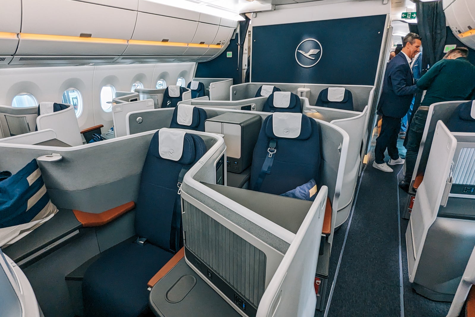
You can book flights, hotels, car rentals, cruises and other travel through Chase Travel, and it's relatively simple to access. First, you'll need to log into your Chase account, then navigate to the right side of the page, where you'll see a little box with your total Ultimate Rewards balance.

Click the box and it will bring you to the Ultimate Rewards dashboard, which looks like this:

Click "Travel" to access the travel homepage and search for airfare, hotels or vacation rentals.

Remember that when you book hotels through the portal with Ultimate Rewards points, you typically will not earn hotel points and elite credits and may not receive elite status perks because it's considered a third-party booking.

However, flights booked through the portal will typically earn frequent flyer miles and qualify for elite status.

How to book flights using Chase Travel

Booking your flights is a straightforward process once you've navigated to the portal's travel page. Type in your arrival and departure airports and travel dates, then hit the search button. For this search, I looked for a one-way flight from San Francisco International Airport (SFO) to Newark Liberty International Airport (EWR).

You'll then see the available flight options. When you find a flight you like, select the fare type you want to book and click the blue "Choose flight" button.

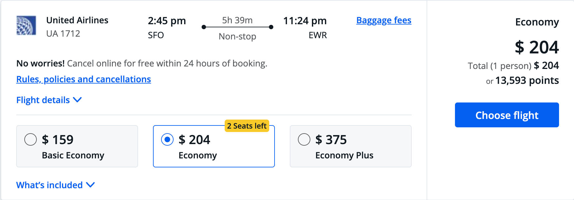
Once you've selected your preferred flights, you'll be taken to the next page to review your flight information and look over any upgrades you'd like to make.

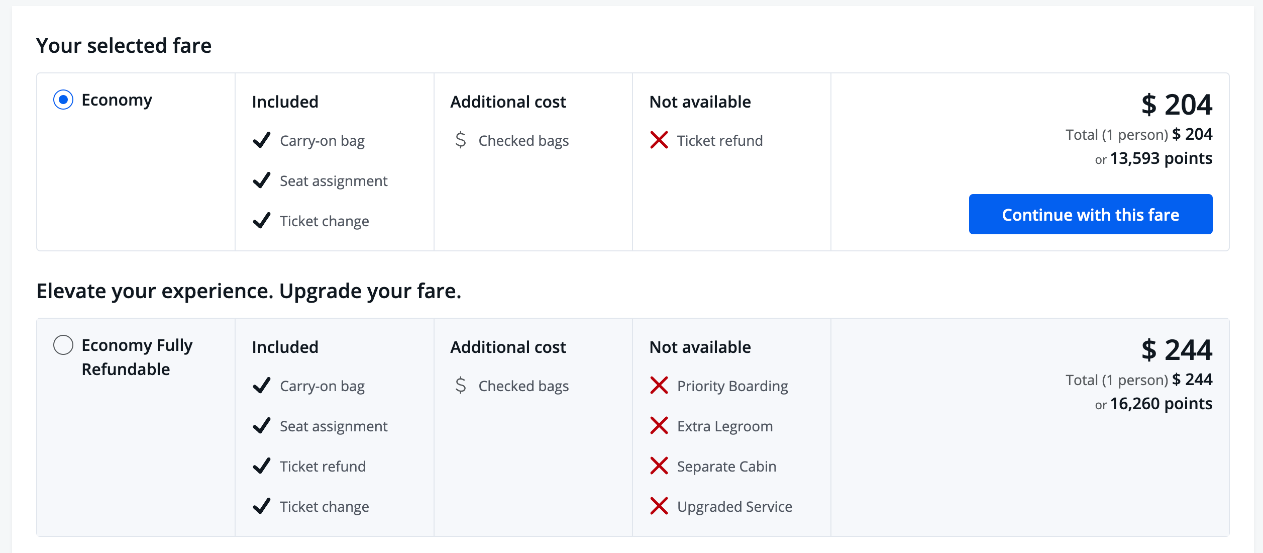
Then, you'll be directed to the checkout page, where you can pay with cash, points or a combination of the two. Again, points linked to a Chase Sapphire Reserve account are worth 1.5 cents each. If you have a Chase Sapphire Preferred Card or Ink Business Preferred Credit Card , points are worth 1.25 cents each.

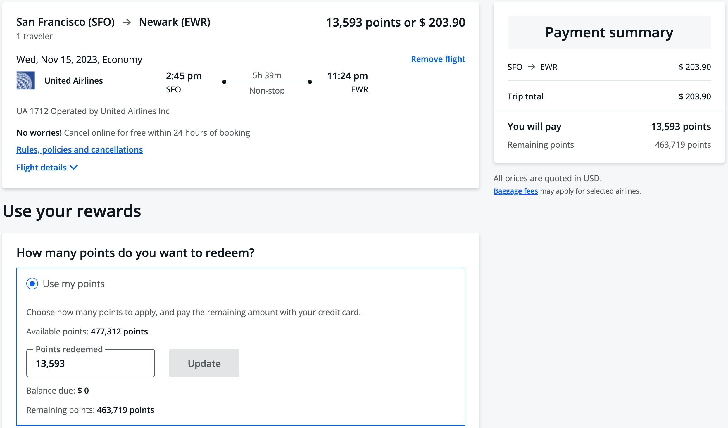
Finally, you'll be directed to a page where you will enter the traveler's information and finalize your flights.

How to book hotels using Chase Travel

Booking hotels is similar to booking flights on the travel portal. This can be advantageous if you're looking at hotels outside of major chains that partner with Ultimate Rewards ( Hyatt , IHG and Marriott ). Regardless of how you book your hotel, compare the award rates required by these hotel loyalty programs to ensure you're getting the best deal.

Also, if you have an eligible card, you can access the Chase Luxury Hotel & Resort Collection , which gives you perks at around 1,000 luxury properties worldwide. Participating cards include the Chase Sapphire Reserve , United℠ Explorer Card , United Club℠ Infinite Card , United Quest℠ Card and United℠ Business Card .

Here's a sample search for hotels in Olso, Norway, which hosts mostly boutique hotels.

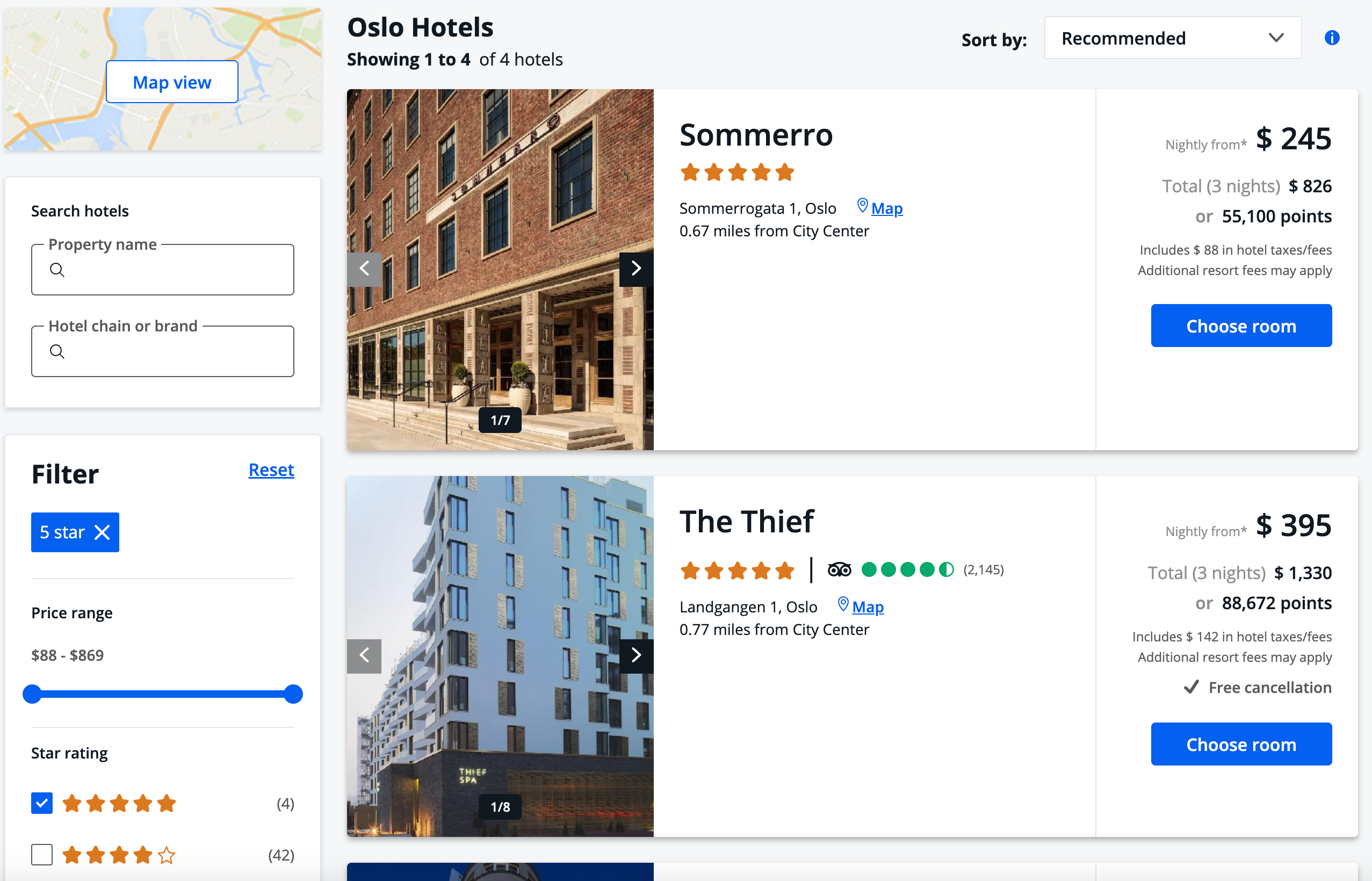
Once you've selected your desired property, room and rate, you can specify how many points you want to use on the checkout page.

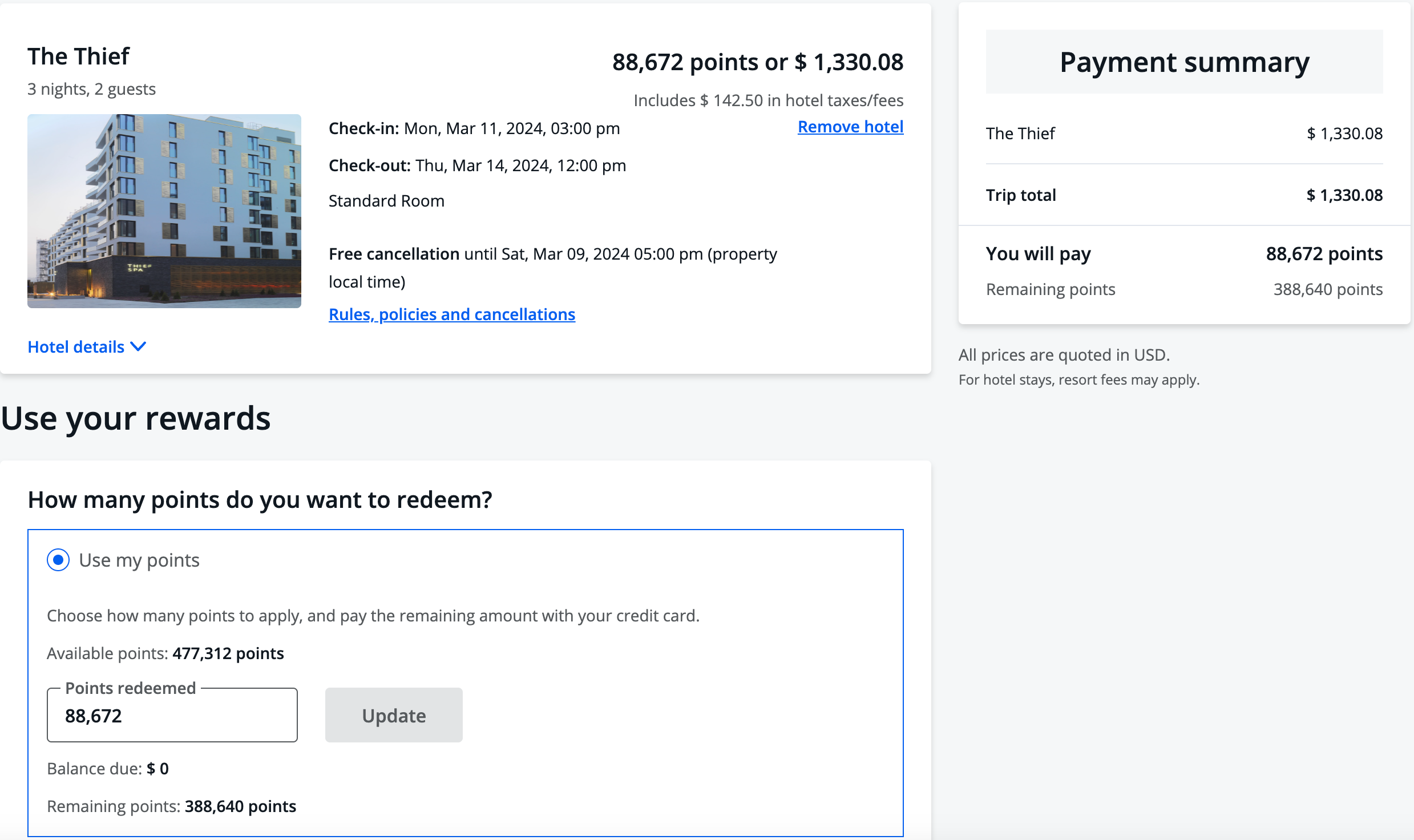
Then, run through the on-screen prompts to finalize your booking, and you'll get an email confirmation.

Remember, you'll receive up to $50 in statement credits yearly for hotel reservations made through Chase Travel as a Sapphire Preferred cardholder.

Related: Book low-end or luxury hotels to get the best value from your points

How to book car rentals, cruises and other travel using Chase Travel

Using Chase Travel, you can rent cars, pay with points and still receive the excellent primary car rental insurance offered by the Chase Sapphire Reserve and Chase Sapphire Preferred Card .

The process of renting cars is similar to booking flights and hotels. Navigate to the "Cars" header from the main landing page and type in your itinerary, even if it's a one-way rental. Then, select "Search," and the results page will pop up. Once you choose your car, you'll be prompted to select add-ons.

When you've finished selecting, you'll head to the booking page, where you'll input your personal information and choose how many points you'd like to spend. Remember that to qualify for rental car insurance, you must decline the car rental company's collision damage waiver and ensure that anyone driving the car is on the rental agreement.

You can also book activities and cruises through Chase. Regarding activities, you can use your points to book fantastic tours like a Washington, D.C., night monument tour or Singapore heritage food tour at 1.25 or 1.5 cents each. This can be an excellent way to make a vacation free, instead of just your hotels and flights.

Cruises are also available, though you'll have to call to book those.

Related: The easiest ways to save on rental cars

More things to consider about Chase Travel

Below is some general guidance to maximize your experience with the portal.

We recommend comparing the points needed through Chase Travel with those required for partner transfers, factoring in taxes and fees. If you have or want hotel elite status, avoid booking hotels through the portal. These stays generally won't count toward status or qualify for hotel elite status benefits.

Booking through Chase Travel with cash can earn you extra points; Ink Business Preferred and Sapphire Preferred cardholders earn 5 points per dollar on all travel and Sapphire Reserve cardholders earn 5 points per dollar on flights and 10 points per dollar on hotels and rental cars. You might find better rates by booking directly with the travel provider; however, if your plans are firm and rates are comparable, booking through the portal can be worthwhile for earning extra points.

Remember that booking through third-party sites may result in issues if you change your plans, though. Travel providers are more likely to assist you if you've booked directly with them.

Bottom line

Chase Travel lets you use your points to book flights, hotels, rental cars, cruises and activities. If award flights aren't available or you find a cheap fare that requires fewer points, booking through the portal can be a good option.

With the Chase Sapphire Preferred and Chase Sapphire Reserve cards offering elevated welcome bonuses of 75,000 Ultimate Rewards points, now is a great time to look at Chase Travel.

Similarly, for hotels, it can be a good deal if you find a cheap rate or book a boutique property, but keep in mind that you may not earn hotel points or receive elite benefits. Whether booking rental cars, activities or cruises, always compare the options to see if using the portal or transferring to partners for an award is more advantageous.

• Investigates
• Houston Life
• Newsletters

WEATHER ALERT

2 warnings and an advisory in effect for 13 regions in the area

Japanese town combating tourists by building screen to block view of mt. fuji, instead of welcoming tourists and the dollars they spend, this town is trying to drive them away.

Keith Dunlap , Digital Content Team, Graham Media Group

Usually towns that are in the middle of a popular tourist spot want to do all they can to cater to tourists.

After all, tourism is usually the lifeblood of the area economy in such towns.

Recommended Videos

However, one town in Japan is actually so fed up with tourists that it’s coming up with a method to drive them away.

Workers in Fujikawaguchiko, a town in the northern foothills of Mt. Fuji, are building a large, black screen along a sidewalk to block the view of the iconic mountain for tourists.

The reason the town is doing this is because they are getting tired of misbehaving foreign tourists, according to The Guardian .

One town official said in the article that tourists have been leaving too much garbage on streets and ignoring traffic regulations.

Since travel restrictions were lifted following the COVID-19 pandemic, tourists have been going in droves to see Mt. Fuji. In March, the number of monthly visitors to Japan exceeded 3 million, according to the article.

Fujikawaguchiko provides a terrific view of Mt. Fuji, with many tourists taking pictures in front of a convenience store that has the mountain as a backdrop.

Evidently though, it’s become too good of a view for the town’s liking, so much so they are taking the unusual step of fighting back against tourists, instead of welcoming them and the money they typically spend.

Graham Media Group 2024

About the Author

Keith dunlap.

Keith is a member of Graham Media Group's Digital Content Team, which produces content for all the company's news websites.